23.2 An Introduction to Fibre Channel, DWDM, and Extended Fabrics We start our discussion with some brief definitions. In the world of HP-UX, sharing storage resources, i.e., disks and tapes over extended distance, will more than likely require us to use Fibre Channel. We implement a Storage Area Network (SAN) as our storage infrastructure. A SAN is a block-based transport architecture; for all intent and purposes, this means it's an interface that can support SCSI protocols. We use Fibre Channel for the following reasons: -
It gives us the extended distances we require. -
We can connect and, hence, share lots of devices -
It provides high bandwidth and low latency. -
It offers reliable transfers of data. -
It is a completely separate physical and logical infrastructure from our IP-based LAN networks, hence, we are not contending with LAN traffic for access to existing bandwidth. A simple explanation of the benefits of Fibre Channel is that it gives us the best of both worlds in terms of the familiarity of SCSI for interfacing with devices, as well as the familiarity of a LAN for extending connectivity over large distances. That's the way I think of Fibre Channel; a SCSI cable that can be miles long with hundreds (possibly millions) of devices connected to it. If that's how you want to think of Fibre Channel, I don't think you will be too far from the truth. I think understanding a SAN as simplistic and manageable is important. I have met many people who consider Fibre Channel and SANs as some form of voodoo cult with arcane rituals, chanting, and dancing around open fires. It isn't. Yes, it's relatively new. Yes, in the early days, getting suppliers to provide hardware that was compatible was nigh impossible (and that's still the case in some instances). Yes, new architecture does mean a new learning curve. But we said that about TCP/IP when it first came out. Look at us now; anyone who doesn't know the difference between a MAC address and an IP address probably needs to read another textbook before reading this one; we take IP addresses for granted these days. So let's reiterate it in as simplistic and manageable a form as we can. A SAN is a miles-long SCSI cable with hundreds of devices connected to it (devices can be disks, tapes, or other servers). Some of you may have come across something called a Network Attached Storage (NAS) device. A NAS device has two major distinctions over a SAN device. A major distinction is that an NAS device offers a file-based transport architecture. Some people I have spoken to said that an NAS-head (a common name for an NAS device that does the front-end processing of requests ) is the natural evolution of a fileserver. NAS devices commonly support CIFS and/or NFS as their underlying filesystem to provide access to files over an existing IP network. The fact that a NAS-device offers a file-based transport architecture sees NAS device more commonly used in a Windows-type infrastructure. That's not to say we can't have NAS devices in a HP-UX infrastructure and vice versa; you could even have an NAS-head that is connected to a collection of disk devices using a backend SAN as their transport infrastructure. We are also seeing SAN protocols being supported over existing IP networks. I suppose the desire to utilize existing IP networks is a cost factor. However, we have to contend with the problem of congestion: Having block-based transport, i.e., SCSI requests, contending with our existing LAN traffic, all over the same infrastructure, must be seen as some form of compromise unless your IP network is offering very high bandwidth, low latency, and possibly even Quality of Service guarantees . For the near future, it seems that HP-UX lives in the world of SANs; it just seems that is the way it has panned out . Fibre Channel is controlled by one of those committees (the NCIS/ANSI T11X3 committee to be precise) that produce those most interesting of documents: standards . In our world of networks, we know about standards and committees; in fact, if we think of the most prevalent model of networking, I would think you would agree it's the OSI seven-layer model. Fibre Channel as a set of standardized protocols is a layered architecture whose design is to transport data across a network. It consists of five layers FC-0 through to FC-4. Figure 23-3 gives you an idea of what each layer achieves. Figure 23-3. Fibre Channel protocol layers. 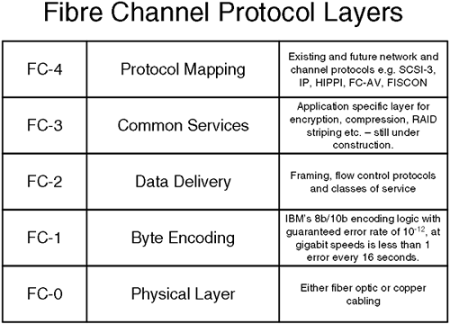
Is this important? In the world of HP-UX, it's not terribly important that we understand every nuance of the standard. We need to get a handle on how this affects managing HP-UX. This includes managing devices files, and setting up, configuring, and managing clusterstwo aspects of managing HP-UX that are immediately affected by implementing a Fibre Channel based SAN. Let's start from the ground up. I'm sure we all think Fibre Channel = fibre- optic , right? Probably, but not necessarily . 23.2.1 Physical medium Fibre Channel standard FC-0 gives us two types of cabling to use: fibre-optic and copper cabling. Fibre optic cabling is the most commonly seen medium because it allows long cable runs. Fibre-optic cable comes in two forms: -
Single-mode fibre : As the name might suggest, this type of fibre carries a light source of a single frequency. This means the cable core can be of a smaller diameter (9 m m = 9 micrometer). Using only a single, long-wave frequency means that we can carry a signal as much as 10km at gigabit speeds. -
Multi-mode fibre : Here we are using multiple short-wave frequencies to transmit a signal. Using multiple frequencies requires a larger cable core. Multi-mode cable uses either a 62.5 m m or 50 m m core. You would think that having considerably more space in the cable core than single-mode fibre would enable us to carry a signal much further. Because of the short wavelength and the dispersion effects caused by using multiple frequencies, we can carry a signal only 175 meters with 62.5 m m cable and 500 meters with 50 m m cable. Both types of cable using 125 m m cladding that the light pulses reflect back into the core. Both types of cable also use a protective outer coating, usually in a distinctive orange color . You can usually determine which type of cable, because the manufacturer's name will be printed on the orange protective coating. The cable/connectors pictured in Figure 23-4 had printed on the orange protective coating "AMP Optical Fibre Cable 50/125" indicating 50 m m core with 125 m m cladding. Because it's such a thin cable, care should be taken not to trap it in suspended -floor tiles in computer rooms: The reflective cladding doesn't work very well with a hole in it. Figure 23-4. SC and LC fibre-optic connectors. 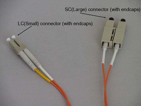
Copper cabling is more commonly used to connect devices (read disks) within rack-mounting cabinets . Consequently, there are two types of copper cable: -
Intracabinet copper : As the name suggest, all connections will be made within one cabinet and uses unequalized cabling limited to 13 meters. -
Intercabinet copper : This is used to connect devices at longer distances, hence intercabinet. It uses active components (signal boosters) to push the signal to distances of up to 30 meters. Currently, we see link speed of either 1 or 2 gigabits; however, 4 gigabits is on the near horizon. Our interface cards and other infrastructure components (that means switches) need to support the desired link speed. An interface card is commonly known as an HBA (host bus adapter). The most common connection between the HBA and the cable is via a GBIC (Gigabit Interface Converter). These are hot-swappable devices about the size of a box of matches. GBICs provide the signal to the physical medium with the HBA performing the serializing/de-serializing (serdes) of the signal. Copper GBICs come in active (up to 30m) and passive (up to 13m) versions using either DB-9 or HSSDC (High Speed Serial Direct Connect) connectors. Optical GBICs come in long wave (up to 10km) and short wave (up to 500m) versions. The power to drive an optical signal to these distances at 2GB/second appears to be a trial for some GBIC manufacturers, and it appears that GBICs running at these speeds seem to fail more than GBICs running at slower speeds. To go beyond 10km, some manufacturers offer Extended Long Wave GBICS that can push a light signal anything from 10km to 40, or even 80km in one hop. As always, developments in this field are fast and furious, with some suppliers claiming single-hop distances in excess of 100km that would normally require the use of Dense Wave Division Multiplexing (DWDM) devices. There are two types of connector for optical GBICs: SC (Standard) connectors or LC (Lucent) connectors. LC connectors are sometimes called SFF (Small Form Factor) connectors. It seems that SC/LC is a common name, and for some perverse, reason it is easier to remember which type of connect is which: -
SC = LARGE connector -
LC = SMALL connector Figure 23-4 should help to remind you: 23.2.2 HBA and WWNs I suppose we will all have to get used to the fact that just about everyone else in the Fibre Channel word calls an interface card a Host Bus Adapter (HBA). I keep referring to them as interface cards, but in mixed company (when you have to speak to non-HP-UX folks), HBA seems to be the most common term . Every HBA has associated with it at least one address known as a WWN. If we take the analogy of a LAN card, every LAN card has (should have) a unique MAC address within a network. In a similar way, every HBA should have a unique identifier within the SAN. Manufacturers obtain a range of identifiers from the IEEE to uniquely identify HBAs from that manufacturer. The identifier comes in two parts : a 64-bit Node Name and possibly a 64-bit Port Name . Because these identifiers are globally unique, they are known as World Wide Names ( WWN ). An HBA will commonly have both a Node WWN and a Port WWN . "Why does it need both?" you ask. The answer is simple. Take a four-port Fibre Channel card. Each individual Port on the card needs to have a unique Port WWN , while the entire card might have a single Node WWN . Here comes the confusing part: -
A node in a SAN is any communicating device, so a node could be a server or a disk. -
A node in a SAN is identified as an N_Port device. -
A node can have many individual connections associated with it; a server can have multiple HBAs, and each HBA may be a four-port Fibre Channel card. -
Every individual connection from a node is associated with an individual N_Port identifier. -
Every individual N_Port has to have a unique WWN associated with it. Got it so far? Okay, so which WWN is used to identify an N_Port device, the Node WWN or the Port WWN ? The answer is that an N_Port is associated with the Port WWN . Remember, the Node WWN may not be unique in the case of a four-port Fibre Channel card, but the Port WWN must be unique . Although the name used, i.e., an N_Port is the Port WWN , may be a little confusing at first, it does make some kind of sense. Someone once tried to liken a Node WWN to a server's hostname and the individual MAC addresses for individual LAN cards as Port WWN s. I suppose that's one way of looking at it. I think the fact that both the Node and Port WWN are of the same 64-bit format also makes it slightly confusing. Just remember that we use the Port WWN in our dealings with SANs and devices. In HP-UX, we can use a command such as fcmsutil to view the Node and Port WWN for our interface cards. First, we need to work out the device files for the individual ports. We do this with ioscan :
root@hp1[] ioscan -fnkC fc Class I H/W Path Driver S/W State H/W Type Description ================================================================= fc 1 0/2/0/0 td CLAIMED INTERFACE HP Tachyon TL/TS Fibre Channel Mass  Storage Adapter /dev/td1 fc 0 0/4/0/0 td CLAIMED INTERFACE HP Tachyon XL2 Fibre Channel Mass Storage Adapter /dev/td0 root@hp1[] Storage Adapter /dev/td1 fc 0 0/4/0/0 td CLAIMED INTERFACE HP Tachyon XL2 Fibre Channel Mass Storage Adapter /dev/td0 root@hp1[]
Here we can see that we have to separate Fibre Channel cards, both with a single Fibre Channel port. The device files being /dev/td0 and /dev/td1 . We can now use fcmsutil to view the Node and more importantly the Port WWN :
root@hp1[] fcmsutil /dev/td0 Vendor ID is = 0x00103c Device ID is = 0x001029 XL2 Chip Revision No is = 2.3 PCI Sub-system Vendor ID is = 0x00103c PCI Sub-system ID is = 0x00128c Topology = PTTOPT_FABRIC Link Speed = 2Gb Local N_Port_id is = 0x010200 N_Port Node World Wide Name = 0x50060b000022564b N_Port Port World Wide Name = 0x50060b000022564a Driver state = ONLINE Hardware Path is = 0/4/0/0 Number of Assisted IOs = 3967 Number of Active Login Sessions = 0 Dino Present on Card = NO Maximum Frame Size = 960 Driver Version = @(#) PATCH_11.11: libtd.a : Jun 28 2002, 11:08 :35, PHSS_26799 root@hp1[] root@hp1[] fcmsutil /dev/td1 Vendor ID is = 0x00103c Device ID is = 0x001028 TL Chip Revision No is = 2.3 PCI Sub-system Vendor ID is = 0x00103c PCI Sub-system ID is = 0x000006 Topology = PTTOPT_FABRIC Local N_Port_id is = 0x010300 N_Port Node World Wide Name = 0x50060b000006be4f N_Port Port World Wide Name = 0x50060b000006be4e Driver state = ONLINE Hardware Path is = 0/2/0/0 Number of Assisted IOs = 2557 Number of Active Login Sessions = 0 Dino Present on Card = NO Maximum Frame Size = 960 Driver Version = @(#) PATCH_11.11: libtd.a : Jun 28 2002, 11:08 :35, PHSS_26799 root@hp1[]
In a simple point-to-point topology, one N_Port would connect directly to another N_Port, i.e., a server would be directly connected to a disk/disk array nice and simple. When we consider other topologies, we realize that the Port WWN is not sufficient to identify nodes in a large complicated SAN. In particular, when we look at Switched Fabric topology, we realize that to route frames through the SAN the Fabric needs the intelligence to identify the Shortest Path from one node to another. It can't do this by just using the Port WWN. The Fabric must use some other identification scheme to identify N_Ports that will allow it to use some form of routing protocol. The routing protocol it uses is known as FSPF (Fibre Shortest Path First) and is a subset of OSPF packet routing in an IP network. Before getting into details about Switched Fabric, let's discuss other topology options. 23.2.3 Topology Fibre Channel supports three topologies: Point-to-Point, Switched Fabric, and Arbitrated Loop. Of the three, Switched Fabric is the most prevalent nowadays. Point-to-Point is simply a server connected to a storage device; this is taking our concept of a mile-long SCSI cable just a little too far! Arbitrated Loop (FC-AL) was common a few years ago while the Switched Fabric products where becoming available. Nowadays, FC-AL is less common. It has lost favor because of its expansion and distance limitations as well as being a shared bandwidth architecture. 23.2.4 FC-AL expansion limitations Although the FC-AL uses a 24-bit address, not all the bits are actually used (the top 16 bits are set to zero). We would assume that the remaining 8 bits could be used for FC-AL addressing giving us 2 8 = 256 addresses. Not so. The requirements of the 8b/10b encoding scheme in FC-1 mean that we only have 127 addresses (known as an AL_PA: Arbitrated Loop Physical Address) available. Each device has a unique address assigned during a Loop Initialization Protocol (LIP) exchange. Some devices have the ability to have their AL_PA set by some hardware or software switches. An AL_PA also reflects the priority of the device: The lower the number, the higher the priority. It would seem that 127 devices is adequate for most small(ish) installations. It is unlikely that you would ever use more than 10-20 devices in a FC-AL environment. One main reason is distance. 23.2.5 FC-AL distance limitations FC-AL is a closed-loop topology. Access to the loop is via an arbitration protocol. As the number of device increases , the chance of gaining access to the loop falls . When you introduce distance into the equation, FC-AL's arbitration can be seen to consume large proportions of the available bandwidth. The Fibre Channel FC-0 standard allows us 10km run of single-mode fibre-optic cable utilizing long-wave transceivers. Light propagates through fibre-optic at approximately 5 nanoseconds/meter. With a 10km run, that equates to a 50-microsecond propagation delay in one direction, or 100-microsecond roundtrip delay. The distance between individual devices calculates the total circumference of the loop. Taking a few 10km runs would consume vast tracks of the available, limited bandwidth; the 100-microsecond delay above equates to 1MB/second in bandwidth terms. It has been shown that beyond 1km FC-AL performance drops of considerably (anything up to 50 percent performance degradation). 23.2.6 FC-AL shared transport limitations Another problem with FC-AL is that it is a shared transport . That is to say, all devices share the available bandwidth . For example, when we get to 50 devices on a 1Gb/second (~100MB/second) Fibre, each device will have on average only 2 MB/second of bandwidth; that's not much. Take a small FC-AL SAN where we have one server connected to a RAID-box of six disks. The RAID-box operates RAID 5 across all disks, and each SCSI disk is operating at approximately 15MB/second. We can see that if the server is providing a service such as streaming video with larger sequential data transfers, all six disks and the server itself are already consuming the entire bandwidth available to FC-AL. Adding more disks would only exacerbate the bandwidth problem, although it would give us more storage. 23.2.7 Loop Initialization Protocol (LIP) Another problem with FC-AL has to do with what happens during a LIP. When a new node joins the loop, it will send out a number of LIPs to announce its arrival and to determine its upstream and downstream neighbors. This seems okay. However, if a node's host bus adapter (HBA; a Fibre Channel interface card to you and me) is faulty and loses contact with the loop, it can get into a situation where it starts a LIP storm . During a LIP, no useful data transmissions can occur. Take a situation with a tape backup. Even with a minor LIP storm, a backup will commonly fail because the device is effectively offline while the LIPs are being processed . Remember that RAID-box we saw previously? If we had to change a faulty disk, this would cause a minor LIP storm, and that's not good . FC-AL commonly utilizes a Loop Hub to interconnect devices. Alternately, you could wire the transmit lead of one node to the receive port of another device, but that's unlikely because adding device into the loop is troublesome ; remember trying to add nodes into a LAN where we used coaxial cable without losing network connectivity for everyone? What a nightmare! Like a LAN hub, a Loop Hub provides a convenient interface to connect devices together. Also like a LAN hub, a Loop Hub has little intelligence other than routing requests between individual ports. Devices connected through a Loop Hub are said to be in a private loop, i.e., they have no notion of anything outside their own little world. The reason for maintaining FC-AL devices is that they may be older devices where the HBA cannot operate in a Switched Fabric configuration. It may be desirable to make these devices available to the rest of the Switched Fabric devices. To be able to do this, the HBA in the device must be able to interact with other Fabric-aware devices. While being able to understand full 24-bit Switch Fabric addresses and perform a Fabric Login (FLOGI) to identify itself within the Fabric, it also must be able to communicate with local loop devices. Not all FC-AL HBAs can exist as public loop devices . If they do support operating as public loop devices, connecting the previously private loop to a Fabric Switch can allow us to migrate the private loop to a public loop . We would plug one of the ports from our Loop Hub into the switch. The switch port will perform a LIP, realize it is participating in a FC-AL, and assume the highest priority AL_PA=0x00; the switch port will operate in a mode known as an FL_port . It is the fact that a private loop is connected to an FL_Port that transforms it into a public loop. In making the private loop a public loop, other devices connected to the Fabric can now communicate with these devices. We also get the benefit of using a Fabric Switch that allows us to maximize the throughput a switch gives us; each port on the switch can support full duplex, 1 or 2Gb/second bandwidth to every other port simultaneously . If the switch port were configured to simply remain a loop port (known as an NL_port ) because the devices on the private loop could not operate in a public loop, these devices would not be accessible via the rest of the Fabric. This is not good for older, legacy devices. The Fibre Channel standards do not care for this situation. It is not a requirement of any Fibre Channel standard to provide Fabric support to non-fabric devices. As you can imagine, customers would find it rather annoying for some standards-body to come along and decree that all your old legacy devices were now defunct ; in order for you to go full-fabric, you would have to upgrade all the HBAs in all your old non-fabric devices. As you can imagine, although it is not a requirement of any standard, many switch vendors support this notion on non-fabric devices being accessible via a fabric. Effectively, the NL_port on the switch will take all requests for the private loop devices and translate the destination ID into a valid address within the Fabric. This mechanism of providing private non-Fabric functionality via multiple switch ports has various names depending on the switch vendor. Supporting private loop on a switch is sometimes known as phantom mode . Other names include stealth mode, emulated private loop ( EPL ), translative mode, and Quickloop . Some switches can support this, but others can't. FC-AL devices communicating in this way are completely unaware of the existence of a Fabric and are therefore still operate as if they were private loop devices. This gets around the problem of non-fabric devices suddenly becoming defunct overnight because we have decided to roll out a Switched Fabric. It allows customers to connect what were separate, standalone private loops into one large virtual private loop . It also allows customers to use older legacy devices within their Fabric until such times as the HBA for that device can be upgraded to be Fabric aware. With all these different topology options, it becomes a challenge for us to identify which ports on a switch are supporting FC-AL , which ones are running in Phantom Mode, and which are supporting Switch Fabric . That will come later. Let's talk a little about Switched Fabric . 23.2.8 Switched Fabric I would have to say that switched fabric is the topology of choice for the vast majority of SAN installations. It alleviates the problems of expansion, distance, and bandwidth seen with FC-AL. A Fabric is a collection of interconnected fabric switches . "Is a SAN a fabric?" you ask. Yes, a SAN can be seen as a Fabric. Remember, a SAN could alternately be a collection of cascading hubs supporting FC-AL, so the topology of Switched Fabric is a topology design decision when constructing a SAN. Because Switched Fabric is the current topology of choice, most people interchange their use of SAN and Fabric and never mind or even understand the difference. Now you know. An individual switch is a non-blocking internal switching matrix that allows concurrent access from one port to any other port. It has anything from 8 to 256 individual ports. Smaller switches are sometimes called edge switches, while large switches are sometimes called core or director class switches due to their high configuration capabilities, extension configuration options, and extremely low latencies (as low at 0.5 m seconds), placing them at the core of a large extended Fabric. There is no formal distinction between a director class and an edge switch; it is more of an arbitrary distinction based on its configuration possibilities. Each port on a switch can operate at full speed and full duplex operation, which means that unlike a Loop Hub that has to share available bandwidth among all connected nodes, as we add more nodes to a switch, performance does not degrade for individual nodes. If you are a marketing-type person, you could even argue that performance increases in direct proportion to the number of nodes attached. This sounds rather suspect, doesn't it? But you can sort of see their point. The aggregate bandwidth of FC-AL does not change; it's a shared bandwidth topology. The aggregate bandwidth of a Switch Fabric will always increase, i.e., eight nodes all communicating a 100MB/second is an aggregate bandwidth of 800MB/second. Add another eight nodes, and your aggregate bandwidth is now 1600MB/second. I told you that you would have to see this through the eyes of a marketer; I suppose I have to concede it is actually a fact. Because each port is operating in concurrent mode with every other node simultaneously, we could almost say the individual communications between nodes are operating like a point-to-point connection. This is not an unreasonable comparison to make; in fact, some devices will designate a Switch Fabric connection as being of the form PP-Fabric, PTTOPT_Fabric, or something similar. The important point is that our interface is fabric aware and able to participate in a Switched Fabric topology. To do this, an HBA must perform a FLOGI or Fabric LOGIn . 23.2.8 SWITCH FABRIC: N_PORT ID When we interconnect switches, we start getting into more complicated territory. First, how does the Fabric know the Shortest Path (remember FSPF ; the subset of the OSPF routing protocol) to an individual N_Port ? When we connect a node to a switch, it goes through an initialization sequence (a bit more of that later). This process, known as FLOGI, is when the node identifies itself to a switch port by sending it a FLOGI frame containing its node name, Port WWN , and what services it can offer (services being things like which protocols a node supports, e.g., SCSI-3, IPv4, IPv6, and so on). At this time, the switch will assign a 24-bit N_Port ID to each node attaching to a port. This 24-bit address space is the same address space used by FC-AL, but unlike FC-AL, which was restricted to 8 bits, Switched Fabric uses the full 24 bits. Some of the addresses are reserved, so from the theoretical 2 24 = 16 million addresses, we can use only 15.5 million. If you are going to have more than 15.5 million nodes connected to your SAN, then you have a problem. As yet, no one has reached this limitation (hardly a surprise!). So we have another address to contend with. Well, I'm afraid that it's the N_Port ID . If we recall the output from the fcmsutil we saw earlier, we can spot the N_Port ID :
root@hp1[] fcmsutil /dev/td1 Vendor ID is = 0x00103c Device ID is = 0x001028 TL Chip Revision No is = 2.3 PCI Sub-system Vendor ID is = 0x00103c PCI Sub-system ID is = 0x000006 Topology = PTTOPT_FABRIC Local N_Port_id is = 0x010300 N_Port Node World Wide Name = 0x50060b000006be4f N_Port Port World Wide Name = 0x50060b000006be4e Driver state = ONLINE Hardware Path is = 0/2/0/0 Number of Assisted IOs = 2557 Number of Active Login Sessions = 0 Dino Present on Card = NO Maximum Frame Size = 960 Driver Version = @(#) PATCH_11.11: libtd.a : Jun 28 2002, 11:08 :35, PHSS_26799 root@hp1[]
It's not as bad as it sounds. We can't change the WWN, and the HBA/port sends the FLOGI frame all by itself. All we need to do is connect them together. The intelligence in the switch assigns an N_Port ID itself. The switch stores the Port WWN to N_Port ID mapping so it knows where you are. This database and the associated service that looks after it are known as the Simple Name Service (SNS). Every switch runs the SNS and maintains its own database of SNS objects . The intelligence in the N_Port ID is that it encodes which switch you are connected to within a Fabric. Not only does it tell you which switch you are connected to, but also which physical port you are connected to. The N-Port ID is a 24-bit address broken down into three 8-bit components of the following form | 23  bits bits  16 16 | 15 bits 8 | 7 bits | | Domain | Area | Port |
At first this might look a little daunting, because there are terms here we haven't met before. Actually, when we put these terms into something a little more understandable, it becomes clear: -
Domain switch number. This means that a Fabric is limited to 2 8 = 256 interconnected switches. In fact, it is limited to 239 interconnected switches because 16 of the addresses are reserved. In reality, a Fabric never gets anywhere near the 239 maximum, although someday someone with lots of money and lots of cable might give it a try. -
Area port number on the switch. -
Port zero in a Switched Fabric; in FC-AL, this is the AL_PA. When we look at the output from fcmsutil , we can see the N-Port ID:
Local N_Port_id is = 0x010300
This now makes sense because we can break this down as follows : -
Domain switch number = 0x01 = Switch number 1. -
Area port number on the switch = 0x03 this HBA is connected to port3 on Switch 1. -
Port = 0x00 = zero in a Switched Fabric; in FC-AL, this is the AL_PA. We can extract the N_Port ID for this HBA by using the command fcmsutil . We could also see this by logging on to the switch and use the command nssshow . When switches are connected together they pass information between each other. Included in this transfer of information is the SNS database maintained on each switch. So, when a server wants to communicate with a disk somewhere within the Fabric, it can query the SNS database on the switch it is connected to and see all devices in the entire Fabric that support the SCSI-3 protocol. When two nodes want to communicate over the fabric, the switches in the Fabric know where they are located because all the switches in the Fabric can query any SNS object connected to the Fabric and resolve its Port WWN to N_Port ID mapping. So far, so good. Plug in a Fibre Channel card to a Fabric Switch and the switch gives its own identifier in order to route packets around the SAN. Easy! In the world of HP-UX, this N_Port ID is actually identifiable in the output from a fcmsutil command, so knowing how an N-Port ID is constructed helps us identify which paths our IO requests are taking through the SAN. In this way, we can evaluate whether we have any SPOFs in our SAN design by identifying individual paths to individual devices (disks). As well as using multiple HBAs, we should also use multiple switches with each HBA connecting into a separate switch. Individual switches can be connected together as well to provide additional paths and additional redundancy. In Figure 23-5, you can see a simple Switched Fabric SAN. In this example, not all connections (the ones to the disk arrays) have full redundancy. This is a less-than -optimal solution. The customer knows and accepts this and is willing to live with it . Figure 23-5. A simple Switched Fabric SAN. 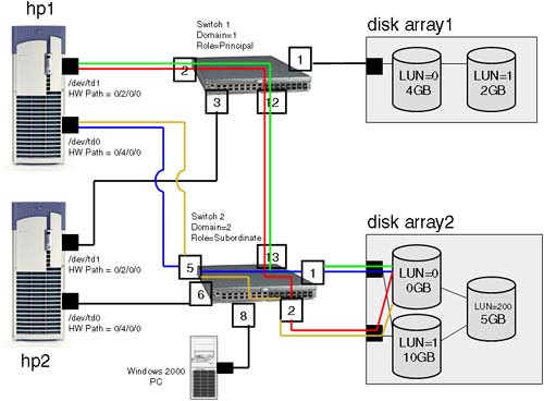
I am only concerned with the connections to LUN0 on disk array 2 . Before we go any further, LUN0 is 0GB in size; it is not a typing mistake. If you want a full discussion on hardware paths and how device files are worked out in a SAN, have a look at Chapter 4: Advanced Peripherals Configuration . Let's return to the discussion at hand. The SNS on each switch will contain a mapping of all devices connected, so when a server wants to communicate with a particular disk, it will query the SNS and be returned the associated N_Port ID of the disk or disk arrays we want to communicate with. As far as HP-UX is concerned, an N_Port ID relates directly to an HP-UX hardware path of the device we are talking toin this case, the disk arrays. Some people find this confusing and expect that the port number of the switch they are attached to and even the switch number they are attached to will somehow be included in the hardware patch seen by HP-UX. Any Inter Switch Links have nothing to do with an HP-UX hardware path for a disk or even a SCSI interface . Another way to look at this is if we go way back to our simplistic view of a SAN, it was a mile-long SCSI cable with hundreds of devices connected to it . If we think about it carefully , the end of our mile-long SCSI cable is going to be the last port we are connected to before we see a disk drive. In this example, our mile-long SCSI cable ends at either port 1 or port 2 on Switch2 . We don't care how we got there; we just care that this is the end of our mile-long SCSI cable . Let's take a look at the hardware paths for the two connections from the server hp1 to LUN0 on disk array 2 (lost of the output from ioscan has been deleted to make this demonstration easier to follow):
root@hp1[] ioscan -fnC disk Class I H/W Path Driver S/W State H/W Type Description ======================================================================== disk 9 0/2/0/0.2.1.0.0.0.0 sdisk CLAIMED DEVICE HP A6189A disk 16 0/2/0/0.2.2.0.0.0.0 sdisk CLAIMED DEVICE HP A6189A disk 13 0/4/0/0.2.1.0.0.0.0 sdisk CLAIMED DEVICE HP A6189A disk 2 0/4/0/0.2.2.0.0.0.0 sdisk CLAIMED DEVICE HP A6189A
For the purposes of this discussion, the format of the hardware path can be broken down into three major components:
<HBA hardware path><N_Port ID><SCSI address>
Let's take each part in turn : <HBA hardware path> : In this case, we have two HBAs on server hp1 , so the hardware path is going to be either 0/2/0/0 or 0/4/0/0 . <N_Port ID> : This is the N_Port ID of the device we are talking to, i.e., the interface for the disk arrays in this case, not the N_Port ID of our HBA . For me, this was something of a breakthrough . Each device is registered on the switch via its WWN to N_Port ID mapping, so the disk array connected to ports 2 and 3 on Switch2 have performed a FLOGI and the switch has associated their Port WWN with an N_Port ID . It is the disk arrays we are communicating with and, hence, it is the N_Port ID of the interfaces on the disk arrays we are concerned with in our HP-UX hardware path. This now starts to make sense. Back in Figure 23-3, we can see that the N_Port ID for all connections to LUN0 are via 2.1.0 or 2.2.0 , which translates to: <SCSI address> : HP-UX hardware paths follow the SCSI-II standard for addressing, so we use the idea of a Virtual SCSI Bus (VSB), target, and SCSI logical unit number (LUN). The LUN number we see in Figure 23-3 is the LUN number assigned by the disk array. This is a common concept for disk arrays. HP-UX has to translate the LUN address assigned by the disk array into a SCSI address. If we look at the components of a SCSI address, we can start to work out how to convert a LUN number into a SCSI address: -
Virtual SCSI Bus : 4-bit address means valid values = 0 through 15. -
Target : 4-bit address means valid values = 0 through 15. -
LUN : 3-bit address mean valid values = 0 through 7. There's a simple(ish) formula for calculating the three components of the SCSI address. Here's the formula: -
Ensure that the LUN number is represented in decimal; an HP XP disk array uses hexadecimal LUN numbers, while an HP VA disk array uses decimal LUN numbers . -
Virtual SCSI Bus starts at address 0. -
If LUN number is < 128 10 , go to step 7 below. -
Subtract 128 10 from the LUN number. -
Increment Virtual SCSI Bus by 1 10 . -
If LUN number is still greater than 128 10 , go back to step 4 above. -
Divide the LUN number by 8. This gives us the SCSI target address. -
The remainder gives us the SCSI LUN. For our example, it is relatively straightforward: -
LUN(on disk array) = 0 10 -
Is LUN number < 128 10 ? If yes, then Virtual SCSI bus = 0 -
Divide 0 by 8 SCSI target = 0 -
Remainder = 0 SCSI LUN = 0 -
SCSI address = 0.0.0 For an explanation of all the examples in Figure 23-3, including a discussion on the associated device files, go to Chapter 4: Advanced Peripherals Configuration. I hope this is starting to make sense. It took me some time to grasp this, but eventually what made the breakthrough was that the concept of the mile-long SCSI cable ending at the last port on the last switch in the SAN gave me the N_Port ID of the device I want to communicate with. The rest of the hardware path was the SCSI components that I could calculate using the formula we saw above. If you have a JBOD (Just a Bunch of Disks) connected to your SAN, the SCSI addressing will be the simple SCSI addresses you set for each device within the JBOD. I was going to finish my discussions on SANs in relation to HP-UX at this point. I decided to go a little further because in an extended cluster environment, we commonly have disks attached via Fibre Channel that are at some distant location. I thought it prudent to discuss some of the technologies you will see to provide an extended SAN. 23.2.9 SANs and port types We start this discussion by looking at the different port types we see in a SAN. This is useful if you ever have trouble communicating with a particular device. If it hasn't performed a FLOGI, it will not be participating in our Switched Fabric and this is a big indication as to why you can't communicate with it. One reason for this is that it may be a Windows-based machine that could be in its own private loop. In fact, this is a common problem for Windows-based machines, because we commonly need to tell the HBA to operate in Switched Fabric mode either via a software setting or by editing the Windows Registry. It is this reliance on software or device driver settings that can make the plug-and-play scenario not work as easily as we first thought. The vast majority of my dealings with HP-UX have been that the device driver you load will determine the topology used by the HBA. Most of the time, we simply need to plug our HBAs into a switch and understand the hardware path we see in ioscan . When this doesn't work, it can be useful to be able to decipher which HBAs are participating in our Switch Fabric and which ones aren't. We can do this by logging in to the switch and seeing which HBAs have registered and what topology they are operating under. Part of the registration/initialization process between the switch and the HBA will determine which topology the HBA is supporting. First, here's an idea of what happens when we connect something into a port on a switch: -
Ports on a switch are known as Universal ports, which means that they can be connected to an Arbitrated Loop, a Switched Fabric, or another switch. -
When two ports are connected, the Universal port on the switch will: -
- Perform a LIP. Essentially , this asks the other port (an HAB possibly) "Are you in an Arbitrated Loop?" If not, proceed to the next stage. -
- Perform a Link Initialization. Essentially, this asks the other port "Are you Switched Fabric?" If not, proceed to the next stage. -
- Send Link Service frames, which essentially means "You must be another switch, so let's start swapping SNS and other information." All this leads to the fact that we have different port types that will allow us to identify which topologies are in force for certain ports on our switch or hub: -
N_Port : A node (server or device) port in a point-to-point or more likely a Switched Fabric. -
NL_Port : A node (server or device) port operating in a FC-AL. -
F_port : A switch port operating in a Switch Fabric. -
FL_port : A switch port operating in FC-AL, connecting a public loop to the rest of the fabric. -
E_Port : An Extension port. (A switch port connected to another switch port. Some switches allow multiple E_Ports to be aggregated together to provide higher bandwidth connections between switches. This aggregation of Inter Switch Links is known as ISL Trunking . To external traffic, the link is seen as one logical link.) -
B_Port : A Bridge port. (This is not seen on a switch but on a device that will connect a switch to a Wide Area Network such as a bridge or router.) -
QL_Port : Sometimes called Phantom, Stealth, or Translative Mode. (QL = Quickloop , which is a Brocade name so check with your switch vendor if they support this functionality. This is not a requirement of any Fibre Channel standard or protocol; it is used by switch vendors to allow customers to connect older non-fabric-aware private loop devices together via a switch. You see QL ports on switches. QL ports allow disparate private loops (loop-lets) to communicate with each other in a large virtual private loop .) -
G_Port : A Generic port. (This is a port on a switch that can operate either as an F_Port or an E_port. You don't normally see G_Ports when looking at a switch.) -
L_Port : A Loop port. (This is a port that can operate in an Arbitrated Loop. Node (NL_port) and fabric (FL_port) are examples of an L_Port. Sometimes, you will see a switch port specifying "L Port public" or "L port private" depending whether it's operating in a Public or Private Loop.) Figure 23-6 is an example of a SAN that has implemented many of the port types listed above. Figure 23-6. An example of SAN port types. 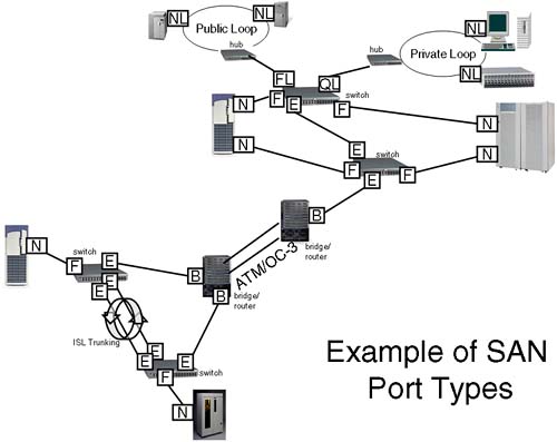
All of the devices in this SAN will be able to communicate with each other except the devices on the Private Loop. With the use of ATM to bridge between sites, this solution could span many miles; it could even span continents. The first thing to mention when we connect switches together is compatibility . It would be helpful if all switches from every vendor could plug-and-play. Currently, this is a nirvana some way off in the distance. In my example in Figure 23-5, I simply plugged port 12 from Switch1 to port 13 of Switch2. The switches negotiated between themselves , and all was well. In a heterogeneous environment, we may have to jump through hoops to get this to work. Incompatibility between switch vendors is probably the main reason customers stick with one switch vendor. This is not to say that switches from the same vendor will automatically work when connected together. Here are some situations I have found myself in that caused same vendor switches not to work straight out of the box: -
Incompatible Domain IDs : Every switch in a Fabric needs to have a unique Switch Domain. If not, the Fabric will become segmented with some switches and devices are not visible. The best solution is to power-up a switch and manually set the Domain ID on every switch. When a switch is introduced into a fabric and it does not have a unique Domain ID, part of the inter-switch negotiation allows for a Domain ID to be re-assigned. If this happens, it may have a detrimental effect on our configured hard zoning . The switch itself may not allow support for the reconfigure fabric link service. Most switches do, but I prefer to ensure that all switches have unique IDs before introducing them into a fabric. -
Incompatible firmware versions : There was a classic problem with versions of firmware on HP/Brocade switches around the time of Fabric OS version 2.7. There was a switch parameter known as "Core Switch PID format." The default prior to Fabric OS version 2.7 was OFF (0=zero). New switches (after Fabric OS version 2.7) had this parameter ON (1=zero). When connecting an old and a new switch together, the Fabric would be segmented. The solution was to change the parameter setting, and all was then okay. Not obvious. Even when we upgraded the firmware on the old switch, the parameter remained the same: contrary to the documentation for the firmware upgrade. So be careful. -
Incompatible port configurations : Switches commonly allow for ports to be configured to allow/disallow certain port types to be configured. If we choose a port that has been configured E_Port_Disallow, then that port is not a good choice to connect two switches together. This needs to be checked on a switch-by-switch basis and a port-by-port basis. Most switches do not disallow port type by default, but it's worth remembering. The easiest way to view port types is to log in to a switch. Most switches will have a 10/100 BaseT network connection that allows you to log in via the network and view/manage port settings. I would suggest you obtain permission from your friendly SAN administrator before doing this because you can make changes to a switch that will render it inoperable in an extended SAN like the example in Figure 23-6. Different switches have different command sets, so it is not easy to give generic examples. The switch I am about to log in to is an HP FC16 switch. It behaves much like a Brocade switch. Here are some example commands to look at port types and extended fabric configurations. To connect to a switch, you will need to know its IP address; otherwise , you will have to connect an RS-232 cable to the DB-9 connector on the front of the switch and onto a terminal/PC. To log in to the switch, you will need to know the administrator's username and password. I hope someone has changed them from being the default of admin/password ! If you refer to Figure 23-5, I have two switches in my Fabric: Switch1 and Switch2 . Here's how I viewed the port types as well as the extent of the Fabric:
Switch1:admin> Switch1:admin> switchshow switchName: Switch1 switchType: 9.2 switchState: Online switchRole: Principal switchDomain: 1 switchId: fffc01 switchWwn: 10:00:00:60:69:51:12:72 switchBeacon: OFF port 0: id N2 No_Light port 1: id N1 Online F-Port 50:06:0b:00:00:1a:0a:6c port 2: id N2 Online F-Port 50:06:0b:00:00:22:56:4a port 3: id N2 Online F-Port 50:06:0b:00:00:22:56:3c port 4: id N2 No_Light port 5: id N2 No_Light port 6: id N2 No_Light port 7: id N2 No_Light port 8: id N2 No_Light port 9: id N2 No_Light port 10: id N2 No_Light port 11: id N2 No_Light port 12: id N2 Online E-Port 10:00:00:60:69:51:4d:b0 "Switch2" (downstream) port 13: id N2 No_Light port 14: id N2 No_Light port 15: id N2 No_Light Switch1:admin> Switch1:admin> fabricshow Switch ID Worldwide Name Enet IP Addr FC IP Addr Name ------------------------------------------------------------------------ 1: fffc01 10:00:00:60:69:51:12:72 155.208.66.151 0.0.0.0 >"Switch1" 2: fffc02 10:00:00:60:69:51:4d:b0 155.208.67.100 0.0.0.0 "Switch2" The Fabric has 2 switches Switch2:admin> switchshow switchName: Switch2 switchType: 9.2 switchState: Online switchMode: Native switchRole: Subordinate switchDomain: 2 switchId: fffc02 switchWwn: 10:00:00:60:69:51:4d:b0 switchBeacon: OFF Zoning: OFF port 0: -- N2 No_Module port 1: id N1 Online F-Port 50:06:0b:00:00:19:6a:30 port 2: id N1 Online F-Port 50:06:0b:00:00:19:65:0a port 3: -- N2 No_Module port 4: -- N2 No_Module port 5: id N1 Online F-Port 50:06:0b:00:00:06:be:4e port 6: id N1 Online F-Port 50:06:0b:00:00:06:c6:c6 port 7: -- N2 No_Module port 8: id N1 Online L-Port 1 public port 9: -- N2 No_Module port 10: -- N2 No_Module port 11: -- N2 No_Module port 12: -- N2 No_Module port 13: id N2 Online E-Port 10:00:00:60:69:51:12:72 "Switch1" (upstream) port 14: -- N2 No_Module port 15: id N2 No_Light Switch2:admin>
Here we can see which Port WWNs are registered against each port. This is not the SNS database, which can be viewed with the nsshow command. To establish which host is connected to which port, we would tally the WWNs from switchshow with the output of fcmsutil run on each server. The 1 L-Port (port 8 on Switch2) is actually a Windows 2000 server. It has to be stressed that the commands used here are specific for the type of switches I am using (HP FC16; similar to Brocade command set). Be sure to check with your vendor which commands are available (typing help after you're logged in to the switch is usually a good start). 23.2.10 Zoning and security One of the last things I want to mention in this (supposedly short) introduction to SANs is the concept of zoning . Refer to the SAN in Figure 23-6 and remember that all devices can communicate with all other devices (except devices in the private loop). This is sometimes a good thing when all servers need to be able to see all devices. However, this is seldom the case in reality. If we attach a Windows-based machine to our SAN and start creating LUNS on our disk arrays, the administrator on the Window-based machine will start to see a number of "Found New Hardware Wizard" screens popping up on his server. Most switches by default have no security enabled; we call this an Open SAN , i.e., everyone can communicate with everyone else's devices. There are basically two forms of security we can implement within a SAN: -
LUN masking : This is the ability to limit access to particular LUNs, e.g., on a disk array, based on the WWN of the initiator. Few switches implement LUN masking. However, many disk array suppliers provide LUN masking software within their own disk arrays, e.g., Secure Manager/XP for HP XP disk arrays. -
Zoning : This is the ability to segregate devices within the SAN. The segregation can be based on departmental, functional, regional, or operating system criteria; it is up to you. The problem we mentioned above regarding our Windows-based server grabbing new LUNs even though they were not destined for that machine would have been resolved by segregating Windows machines and their storage devices away from HP-UX machines and their storage devices. For example, we could have all HP-UX machines and their storage devices in an HP-UX zone with the Windows machines in a Windows zone. Zones can overlap, e.g., a TapeSilo zone for all our tape storage devices. HP-UX machines could belong to both an HP-UX and a TapeSilo zone to allow them to perform tape backups . The same could be true for the Windows zone. A zone is a "collection of members within a SAN that have the need to communicate between each other." When I use the word member, I do so for a reason. A member can be either: This gives us two options in how we implement zoning. Each type of zoning has pros and cons: Because zoning and security are becoming key features within a SAN, interoperability between vendors is becoming more and more common (although no guarantees can be given at this stage). Let's look at an example of the two switches I showed you earlier in Figure 23-5. Currently, there is no zoning in place, i.e., both servers can see all the LUNs configured on both disk arrays. If I wanted to implement zoning, I would have to sit down with my diagram and work out which members wanted to communicate with each other. I prefer hard zoning , primarily because of the security implications. In this example, my planning is relatively simple: With hard zoning, we need to work out which physical ports on particular switches need to communicate. Remember, the physical ports are our members in hard zoning . I can now give my zones names and assign ports to those zones. Ports are normally named <switch domain>,<port number> , e.g., 2,5 for switch domain = 2, port number = 5. The switch domain you can get from the output of the switchshow command. I hope we have established which servers are connected to which ports by tallying the WWN from the command fcmsutil with the output from switchshow . Here are the zones I have worked out: Most switches allow you to configure aliases for members. For example, hp1td0 could be an alias for member 2,5, in other words, the connection from server hp1 to the switch via Fibre Channel interface /dev/td0 . This can make your configurations much easier to understand but is not obligatory . Another thing to watch is that some switch vendors may require you to include E_Ports into your zones. In this case, I would need to include member 1,12 and 2,13 into both zones. With my particular switches, this is not necessary. Once you have planned out your zoning, it is time to start configuring it. Here is my cookbook approach to setting up zoning (I have included the commands I used on my switches for demonstration purposes): -
Establish which switch is the Principal Switch in your Fabric. The Principal Switch assigns blocks of addresses to other switches in the fabric to ensure that we do not have duplicate addresses within the Fabric. The selection of a Principal Switch is part of the inter-switch negotiation. Using the switchshow command shows you the SwitchRole (see output above). In my two-switch Fabric, it so happens that Switch1 is the Principal Switch. Using the Principal Switch to configure zoning ensures that all configuration changes are propagated to all Subordinate Switches .
-
Set up any aliases you will use for nodes in the Fabric. Switch1:admin> alicreate "hp1td0","2,5" Switch1:admin> alicreate "hp1td1","1,2" Switch1:admin> alicreate "hp1RA1CH1","1,1" Note for my naming convention : hp1RA1CH1 hp1 = server name RA1 = disc array1 CH1 = channel 1 (interface on disc array) Switch1:admin> alicreate "hp2td0","2,6" Switch1:admin> alicreate "hp2td1","1,3" Switch1:admin> alicreate "hp2RA2CH1","2,1" Switch1:admin> alicreate "hp2RA2CH2","2,2 " -
Establish individual zones. Switch1:admin> zonecreate "hp1DATA","hp1td0; hp1td1; hp1RA1CH1" Switch1:admin> zonecreate "hp2DATA","hp2td0; hp2td1; hp2RA2CH1; hp2RA2CH2" -
Establish a configuration . A configuration is a collection of independent and/or overlapping zones. Only one configuration can be enabled at any one time. Switch1:admin> cfgcreate "HPUX", "hp1DATA; hp2DATA" -
Save and enable the relevant configuration . Switch1:admin> cfgsave Updating flash ... Switch1:admin> cfgshow Defined configuration: cfg: HPUX hp1DATA; hp2DATA zone: hp1DATA hp1td0; hp1td1; hp1RA1CH1 zone: hp2DATA hp2td0; hp2td1; hp2RA2CH1; hp2RA2CH2 alias: hp1RA1CH1 1,1 alias: hp1td0 2,5 alias: hp1td1 1,2 alias: hp2RA2CH1 2,1 alias: hp2RA2CH2 2,2 alias: hp2td0 2,6 alias: hp2td1 1,3 Effective configuration: no configuration in effect Switch1:admin> cfgenable "HPUX" zone config "HPUX" is in effect Updating flash ... Switch1:admin> -
Check that configuration has been downloaded to all Subordinate Switches . Switch2:admin> Switch2:admin> cfgshow Defined configuration: cfg: HPUX hp1DATA; hp2DATA zone: hp1DATA hp1td0; hp1td1; hp1RA1CH1 zone: hp2DATA hp2td0; hp2td1; hp2RA2CH1; hp2RA2CH2 alias: hp1RA1CH1 1,1 alias: hp1td0 2,5 alias: hp1td1 1,2 alias: hp2RA2CH1 2,1 alias: hp2RA2CH2 2,2 alias: hp2td0 2,6 alias: hp2td1 1,3 Effective configuration: cfg: HPUX zone: hp1DATA 2,5 1,2 1,1 zone: hp2DATA 2,6 1,3 2,1 2,2 Switch2:admin> -
Test that all servers can still access all their storage devices.
On HP-UX, this will require checking that all disks and tapes are still visible by using the ioscan command: Make sure that you do not use the -k option, which will only query the kernel. Not using the k option means that ioscan will actually probe the available hardware. If you seen any NO_HW against a device, it means your server has lost contact with that device. Check that your zoning is doing what it supposed to do. If not, you will have to revise it to ensure that all servers can see the relevant hardware. Also check that servers cannot see devices they are not supposed to see.
23.2.11 Extended Fabricsmore switches Connecting multiple switches together can be a challenge in itself due to vendor and other interoperability reasons. Theoretically, we can interconnect 239 switches to form a single Fabric. Most Fabrics these days seldom extend beyond 10-20 switches. The latencies involved between switches can become an issue, hence, the reason for using Director Class switches at the core of your Fabric configuration that have extremely low latencies. Even though the routing protocol used for inter-switch routingFSPFis a link state (least cost) routing protocol, some vendors suggest limiting (and in some cases, they limit) the maximum number of hops between servers and storage devices. One reason for this is that FSPF only uses a cost metric (very primitive formula) for calculating the cost of a particular link. In the near future, we may see (in FSPF version 2) a latency parameter that may be used in the cost calculation. In this way long, distance routes will be less attractive than routes with less latency. 23.2.12 Extended Fabrics long distances Another aspect of implementing an extended fabric is accommodating long distances. As mentioned earlier, we can utilize Extended GBICs to push a light pulse beyond 10km, sometime even to 120km in a single hop. The first thing we need to link about is the speed of light. Yep, this starts to become a factor. A Fibre Channel frame is approximately 2KB (2148 bytes) in size. It may seem strange that 2KB equates to 2148 bytes. This is due to the encoding scheme used by Fibre Channel (FC-1). The encoding scheme is known as 8b.10b encoding scheme where a byte is 10 bits. Imagine if we were to look at a window in a fibre (operating at 1Gb/second) that was exactly one frame in size and time how long a single Fibre Channel frame took to enter and leave our window ; it would take approximately 20 m seconds (0.00002 seconds) from the first bit of the frame entering the window until the last bit leaves the window . So let's talk distances now. How long is a frame within a fibre? This may seem a strange question, but stay with it. The speed of light in a vacuum is 299.792.458 meters/second. I hope you don't mind my rounding that to 300.000.000 meters/second = 300.000 Km/second (if you are an Empirical junkie that = 186,000 miles/second). Now, in a fibre, light doesn't travel that fast; we have to account for the density of the fibre. The refractive index of glass is 1.5. This means that the speed of light in a fibre is 200.000 km/second (or a latency of 5 nanoseconds per meter). If a frame takes 0.00002 seconds (20 m seconds) to propagate through a fibre, that means a single frame is 200.000 x 0.00002 = 4Km (2.5 miles) in length. If we take our standard 1Gb/second GBIC that can operate over 10Km, it can pump 2.5 frames into the fibre before they reach the other end. This is known as the propagation delay, and we need to consider it in a SAN that involves multiple devices and long distances. If we take a simple configuration where we have one server, one switch, and one destination device, we can work out the propagation delay in the roundtrip time to send a single frame through our SAN. The resulting figure is known as buffer credits . Devices and nodes will establish their buffer credits (known as buffer-to-buffer credit BB_Credit ) as part of the login process with the switch. Before a device sends a frame to a switch or vice-versa, it checks the buffer credits available for that device. If there are no credits available, the frame cannot be sent. Not having enough BB_Credits available for a single link would be a major performance problem because the devices were not operating optimally; in a 100Km link, we can fit 25 frames into the fibre before the first frame reaches the distant device. Most switch ports have a setting that automatically allows for enough BB_Credits for a single 10Km link. Once we go beyond a 10Km link, we may have to start increasing the BB_Credits for a given switch and individual switch ports. Figure 23-7 shows a simple example of Propagation delays in a 1Gb fibre and the associated BB_Credits required. Figure 23-7. Propagation delays in a 1Gb fibre. 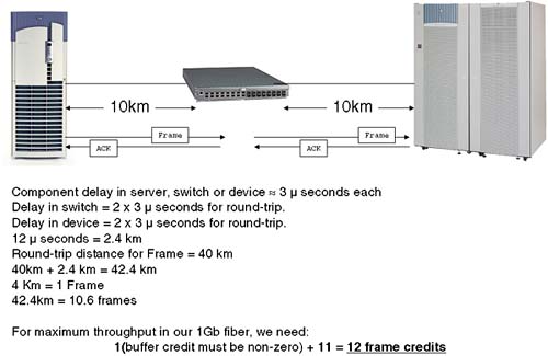
In the case of the switches I am using (HP FC16 switches), there is a port setting known as portCfgLongDistance , which can be set to one of three values: 0 = up to 10Km, 1 = up to 50Km, or 2 = 100Km. You need to check a number of things before setting this: -
There is usually a Long Distance setting (similar to above) for the entire switch. This will require you to disable the switch before changing the setting. -
Which ports can be set for Long Distance? Some switches group a number of consecutive ports onto a single ASIC (Application Specific Integrated Circuit) known as a loom . If we have four ports per loom, I would normally only be able to configure one port per loom as a Long Distance Port. -
Configure all switches in the Fabric as Long Distance; otherwise, the Fabric will become segmented. -
To increase BB_Credits is very seldom free; if you can afford long runs of fibre, then you can afford to pay the switch supplier for some more buffer credits. Remember to install the Long Distance license on all switched in the Fabric. As you can see, long distances causes some configuration changes, and having ports communicating over +10Km will require an increase in your BB_Credits allowance on all your switches. The costs don't stop there. 23.2.13 Installing your own fibre: dark fibre, DWDM, and others We have been discussing the possibility of running Fibre Channel over distances up to and in excess of 10Km. This requires one fundamental piece of hardware: fibre-optic cable. I was talking to a customer in the UK recently who was considering running a private fibre over a distance of 30Km. The cost he was quoted for simply installing the fibre was approximately $7.5 million. That was for two individual fibres running in the same underground conduit. The customer immediately pointed out that having both fibres in the same conduit was not the best idea from a High Availability standpoint. To install two separate fibres was going to at least double the cost. Allied with this is the problem of access. You will need to gain access to the land you intend to run the fibre through. This can a considerable additional cost in terms of paying for access rights as well as the legal fees to administer such an undertaking. As you can imagine, few customers are laying their own fibre. The UK has an abundance of TV-cable companies that have taken the time, effort, and expense to lay fibre-optic cable all over the country. Lots of this fibre has no light signal going through it. This is known as dark fibre , simply because of the fact no light pulses are being sent down the fibre. As we have just discussed, laying your own fibre is expensive. Companies that have dark fibre are keen to recoup their investment costs. One way they can do this is to sell or lease you capacity on a dark fibre. If you wanted the bandwidth capabilities of an entire fibre all to yourself, I am sure they would charge you handsomely for the privilege. A common solution is to multiplex multiple optical frequencies down a fibre (using a standby fibre is a good idea for High Availability reasons) allowing multiple signals potentially from multiple sources to take advantages of the bandwidth potential of fibre. This solution is known as Dense Wave Division Multiplexing ( DWDM ). This solution involves leasing space or actually a frequency on a fibre from a telecom supplier. To attach to the fibre, you will connect through a DWDM device. The DWDM device may be housed on your site, or you may have to run fibre to the DWDM device itself. Either the telecom supplier or the DWDM supplier will normally ensure that the DWDM ports are installed and configured with appropriate converters for your type of connection: high speed converters for Fibre Channel, low speed converters for 100BaseFX Ethernet). The connections between the DWDM devices will be via long-wave GBICs over single-mode fibre. It's probably a good idea to ensure that as part of your agreement the telecom supplier is providing a redundant link in case a single cable fails. With more and more customers wanting to shift data long distances using Fibre Channel, lots of people have regarded DWDM as solely a feature of Fibre Channel SANs. It has become associated with Fibre Channel purely out of market forces. There is nothing to stop an organization running IP protocols over a DWDM link; it can support multiple protocols simultaneously. The great thing about using a DWDM device is that in a SAN it is simply seen as an extension port, an E_Port. This means we can plug a switch, a node, or even a storage device port directly into our DWDM device and visualize it as if we would any other switch in the Fabric. Well, almost. Once we start thinking about these kinds of distances, we need to start thinking about propagation delays. The DWDM devices will normally have huge bandwidth potential, but no matter how much data they can handle, they will introduce propagation delays due to internal circuitry as well as delays due to the length of the fibre they are attached to. Figure 23-7 above started the discussion regarding propagation delays in relation to BB_Credits. We also need to consider the propagation delays in regard of actual time scales . Let's look at an example: -
We have a pair DWDM devices from a reputable manufacturer such as CNT (http://www.cnt.com UltraNet Wave Multiplexer) or ADVA Optical (http://www.advaoptical.com ADVA FSP-II). The latency from the single DWMD device is something approaching 250 nanoseconds = 2 x 250 ns = 500 ns latency. -
Light in fibre travels at 200.000Km/second which equates to a latency = 5 ns. -
- A 50Km fibre = 50.000 * 5 ns = 250.000 ns latency. -
Most applications, e.g., disk writes require a confirmation of the write, hence, the total latency is doubled . Latency = 2 x ((250 ns x 2) + (50.000 x 5 ns)) = 0.501 ms This is simply the latency introduced by the DWDM devices and the 50Km of fibre. We also need to consider any additional latency in connecting our servers and devices into our SAN. Such figures need to be considered when configuring software such as remote data replication software, which commonly has timeout values associated with getting a response from remote devices. DWDM links have been seen to run successfully over 10s of kilometers, in some cases up to 100Km. If distances beyond this are required, we may need to consider other solutions. 23.2.14 Fibre Channel bridges Once we go beyond what we could call metropolitan distances, we need to consider utilizing other wide area network (WAN) solutions. These will be supplied by telecom suppliers in the form of access to a high bandwidth network such as ATM. We will need to provide some hardware to connect to such a network. This device will be our bridge from Fibre Channel to the WAN; it will take Fibre Channel frames and break them up into ATM frames, reassembling them at the remote location. In our picture of our SAN, these ports will be seen as B_Ports. Companies such as CNT (http://www.cnt.com) provide products that perform such a task. For extended Cluster solutions, you will need to check with Hewlett-Packard which combinations of products are currently supported (CNT and CISCO are high on this list). The configuration of the bridge is normally within the remit of the supplier and/or the telecom company. We need to ensure that we have adequate bandwidth over the link and that we have paid for redundancy should there be a problem with connections to the WAN itself. Most bridge devices offer high availability features such as hot-swappable components and redundant internal devices. We should consider the possibility of such a device suffering a catastrophic failure itself. If we want to maximize the uptime of this solution, we may need to either (a) buy multiple bridges or (b) lease connections on bridges supplied by telecom suppliers and ensure that our contract stipulates 100 percent availability. These solutions are never cheap, and the cost increases exponentially with the bandwidth we require. Our bandwidth requirements will depend on the types of applications we are running over the link. Providing high-definition video (  150MB/second) over a T1 link is not going to provide adequate performance. Knowing what solutions your telecom supplier is offering and at what cost is important. Here are some bandwidth figures for common WAN solutions: 150MB/second) over a T1 link is not going to provide adequate performance. Knowing what solutions your telecom supplier is offering and at what cost is important. Here are some bandwidth figures for common WAN solutions: | Service (US telecom) | Link Speed | | DS1/T1 | 1.544 Mb/second | | DS3/T3 | 54 Mb/second | | OC-3c | 155 Mb/second | | OC-12c | 622 Mb/second | | OC-48c | 2.5 Gb/second | | OC-192c | 10 Gb/second |
| Service (USA telecom) | Link Speed | | E1 | 2.048 Mb/second | | E3 | 34 Mb/second | | STM-1 | 155 Mb/second | | STM-4 | 622 Mb/second | | STM-16 | 2.5 Gb/second | | STM-64 | 10 Gb/second |
Although these figures look exciting, we need to consider two things: -
The data rate (sometime called payload rate), which excludes any network- related headers, is commonly considerably less than the link speed, e.g., the data rate for STM-64/OC-192c 8.6 GB/second. |