The Anatomy of a Multiple Consolidation Range Pivot Table

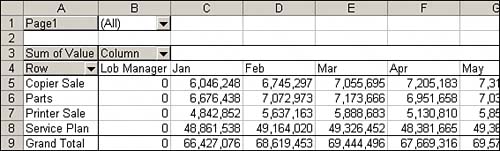
After closer analysis of your new pivot table, you will notice a few interesting things. First, your field list includes a field called Row, a field called Column, a field called Value, and a Field called Page1.

It is important to keep in mind that pivot tables using multiple consolidation ranges as their data source can only have three base fields: Row, Column, and Value. In addition to these base fields, you can create up to four page fields.

TIP

You will notice that the fields generated with your pivot table have fairly generic names (Row, Column, Value, Page). You can customize the field settings for these fields to rename and format them in order to better suit your needs. See Chapter 3, "Customizing Fields in a Pivot Table," for a more detailed look at customizing field settings.

The Row Field

The Row field is always made up of the first column in your data source. Note that in Figure 8.2, the first column in your data source is line of business. Therefore, the Row field in your newly created pivot table contains line of business.

The Column Field

The Column field contains the remaining columns in your data source. Pivot tables that use multiple consolidation ranges combine all the fields in your original datasets (minus the first column, which is used for the Row field) into a kind of super field called the Column field. The fields in your original datasets become data items under the Column field.

As you will notice in Figure 8.10, your pivot table initially applies Count to your Column field. If you change the field setting of the Column field to Sum, all the data items under the Column field are affected.

Figure 8.10. The data items under the Column field are treated as one entity. When you change the calculation of the Column field from Count to Sum, the change applies to all items under the Column field.

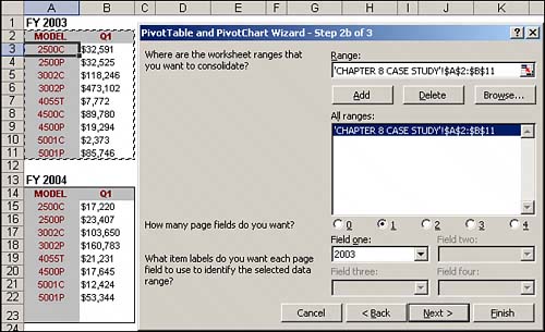
The Value Field

The Value field contains the value for all data items under the Column field. Notice that even fields that were originally text fields in your dataset are treated as numerical values. An example is Lob Manager, shown in Figure 8.10. Although this field contained manager names in the original dataset, it is now treated as a number in your pivot table.

As mentioned before, pivot tables that use multiple consolidation ranges merge the fields in your original datasets (minus the first field), making them data items in the Column field. Therefore, although you may recognize fields such as Lob Manager as text fields that contain their own individual data items, they no longer hold data of their own. They have been transformed into data items themselvesdata items with a value.

The net effect of this behavior is that fields originally holding text or dates show up in your pivot table as a meaningless numerical value. It's usually a good idea to simply hide these fields to avoid confusion. See Chapter 5, "Controlling the Way You View Your Pivot Data," for a more detailed look at hiding fields.

The Page Fields

Page fields are the only fields in a multiple consolidation range pivot tables that you have direct control over. You can create and define up to four page fields. The useful thing about these fields is that you can drag them to the row area or column area to add layers to your pivot table.

The Page1 field shown in the pivot table in Figure 8.10 was created to be able to filter by region. However, as you can see in Figure 8.11, if you drag the Page1 field to the row area of your pivot table, you can create a one-shot view of all your data by region.

Figure 8.11. Dragging the Page1 field to the row area adds a layer to your pivot table report, giving you a one-shot view of all your data by region.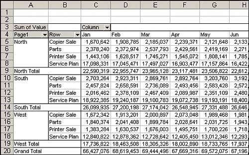

Redefining Your Pivot Table

You may run into a situation where you need to redefine your pivot tablethat is, add a data range, remove a data range, or redefine your page fields. To redefine your pivot table, simply right-click anywhere inside your pivot table, select PivotTable Wizard, and then click the Back button until you get to the dialog box you need.

CASE STUDY: Consolidate and Analyze Eight Datasets

Your manager has forwarded you the spreadsheet shown in Figure 8.12 and has asked you to extract a two-year average revenue by quarter for each model number. Your manager requires these figures for a meeting that starts in 15 minutes, so you have very little time to organize and summarize this data.

Figure 8.12. You need to analyze the data in this spreadsheet and quickly extract the two-year average revenue by quarter for each model number.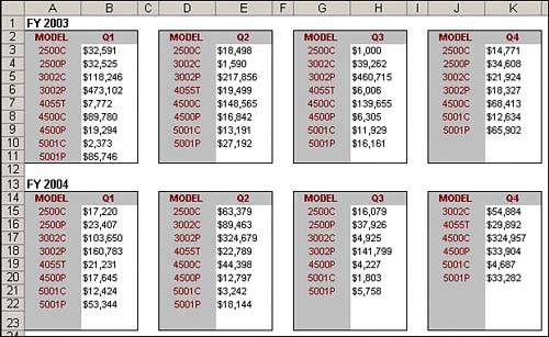

Given that this is a one-time analysis that needs to be completed quickly, you decide to use a pivot table. Here are the steps you will follow:

1.	Start the PivotTable Wizard and select Multiple Consolidation Ranges as your data source. Click Next.
2.	Select the I Will Create the Page Fields option and then click Next.
3.	Add your first data range and then select the radio button next to the number 1 to activate the Field One input box. Enter "2003" into the input box.
At this point, your dialog box should look like Figure 8.13. Figure 8.13. After you add your first data range, your dialog box should look like this.
4.	Add your second data range and enter "2003" into the input box.
5.	Repeat step 4 for each of your datasets until you have added all your data ranges. Be sure to enter "2004" for all the datasets that are under FY 2004.

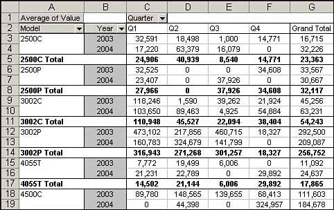
At this point, your dialog box should look like Figure 8.14.

Figure 8.14. After all your data ranges have been added, click Finish to finalize your pivot table.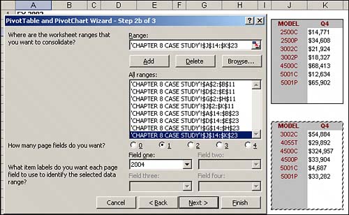

You have successfully consolidated your data into one pivot table! However, as you can see in Figure 8.15, you will have to change the field settings on your Value fields to calculate Average instead of Count. In addition, you will want to rename the fields in your pivot table to better define your data.

Figure 8.15. After your pivot table has been generated, you will need to change the field settings on your Value fields to calculate Average instead of Count.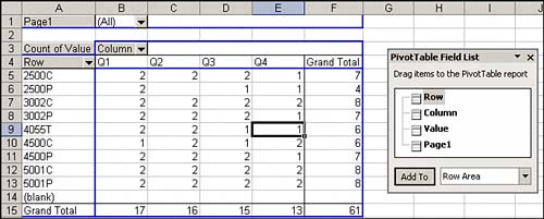

After you apply the necessary formatting changes, your pivot table should look similar to the one shown in Figure 8.16. With this streamlined structure, you are showing the optimal amount of data in an easy-to-read format.

Figure 8.16. With your reorganized pivot table report, you have provided your manager with a report that shows the average revenue for each model number by quarter, by year, and as a two-year average.