7.2 Arrays
7.2 Arrays
After strings, arrays are probably the most common composite data type (a complex data type built up from smaller data objects). Yet few beginning programmers fully understand how arrays operate and know about their efficiency trade-offs. It's surprising how many novice programmers view arrays from a completely different perspective once they understand how arrays operate at the machine level.
Abstractly, an array is an aggregate data type whose members (elements) are all of the same type. A member is selected from the array by specifying the member's array index with an integer (or with some value whose underlying representation is an integer, such as character, enumerated, and Boolean types). This chapter assumes that all of the integer indexes of an array are numerically contiguous (though this is not required). That is, if both x and y are valid indexes of the array, and if x < y , then all i such that x < i < y are also valid indexes. In this book, we will assume that array elements occupy contiguous locations in memory. An array with five elements will appear in memory as shown in Figure 7-2.
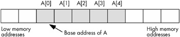
Figure 7-2: Array layout in memory
The base address of an array is the address of the first element of the array and is at the lowest memory location. The second array element directly follows the first in memory, the third element follows the second, and so on. Note that there is no requirement that the indexes start at zero. They may start with any number as long as they are contiguous. However, for the purposes of this discussion, it's easier to discuss array access if the first index is zero. We'll generally begin most arrays at index zero unless there is a good reason to do otherwise .
Whenever you apply the indexing operator to an array, the result is the unique array element specified by that index. For example, A[i] chooses the i th element from array A .
7.2.1 Array Declarations
Array declarations are very similar across many high-level languages. We'll look at some examples in many of these languages within this section.
C, C++, and Java all let you declare an array by specifying the total number of elements in an array. The syntax for an array declaration in these languages is as follows:
data_type array_name [ number_of_elements ];
Here are some sample C/C++ array declarations:
char CharArray[ 128 ]; int intArray[ 8 ]; unsigned char ByteArray[ 10 ]; int *PtrArray[ 4 ];
If these arrays are declared as automatic variables , then C/C++ 'initializes' them with whatever bit patterns happen to be present in memory. If, on the other hand, you declare these arrays as static objects, then C/C++ zeros out each array element. If you want to initialize an array yourself, then you can use the following C/C++ syntax:
data_type array_name [ number_of_elements ] = { element_list }; Here's a typical example:
int intArray[8] = {0,1,2,3,4,5,6,7}; HLA's array declaration syntax takes the following form, which is semantically equivalent to the C/C++ declaration:
array_name : data_type [ number_of_elements ];
Here are some examples of HLA array declarations, which all allocate storage for uninitialized arrays (the second example assumes that you have defined the integer data type in a type section of the HLA program):
static CharArray: char[128]; // Character array with elements // 0..127. IntArray: integer[ 8 ]; // Integer array with elements 0..7. ByteArray: byte[10]; // Byte array with elements 0..9. PtrArray: dword[4]; // Double-word array with elements 0..3.
You can also initialize the array elements using declarations like the following:
RealArray: real32[8] := [ 0.0, 1.0, 2.0, 3.0, 4.0, 5.0, 6.0, 7.0 ]; IntegerAry: integer[8] := [ 8, 9, 10, 11, 12, 13, 14, 15 ];
Both of these definitions create arrays with eight elements. The first definition initializes each 4-byte real32 array element with one of the values in the range 0.0..7.0. The second declaration initializes each integer array element with one of the values in the range 8..15.
Pascal/Delphi/Kylix uses the following syntax to declare an array:
array_name : array[ lower_bound..upper_bound ] of data_type ;
As in the previous examples, array_name is the identifier and data_type is the type of each element in this array. Unlike C/C++, Java, and HLA, in Pascal/Delphi/Kylix you specify the upper and lower bounds of the array rather than the array's size . The following are typical array declarations in Pascal:
type ptrToChar = ^char; var CharArray: array[0..127] of char; // 128 elements IntArray: array[ 0..7 ] of integer; // 8 elements ByteArray: array[0..9] of char; // 10 elements PtrArray: array[0..3] of ptrToChar; // 4 elements
Although these Pascal examples start their indexes at zero, Pascal does not require a starting index of zero. The following is a perfectly valid array declaration in Pascal:
var ProfitsByYear : array[ 1998..2009 ] of real; // 12 elements
The program that declares this array would use indexes 1998 through 2009 when accessing elements of this array, not 0 through 11.
Many Pascal compilers provide an extra feature to help you locate defects in your programs. Whenever you access an element of an array, these compilers will automatically insert code that will verify that the array index is within the bounds specified by the declaration. This extra code will stop the program if the index is out of range. For example, if an index into ProfitsByYear is outside the range 1998..2009, the program would abort with an error. This is a very useful feature that helps verify the correctness of your program. [1]
Generally, array indexes are integer values, though some languages allow other ordinal types (those data types that use an underlying integer representation). For example, Pascal allows char and boolean array indexes. In Pascal, it's perfectly reasonable and useful to declare an array as follows:
alphaCnt : array[ 'A'..'Z' ] of integer;
You access elements of alphaCnt using a character expression as the array index. For example, consider the following Pascal code that initializes each element of alphaCnt to zero:
for ch := 'A' to 'Z' do alphaCnt[ ch ] := 0;
Assembly language and C/C++ treat most ordinal values as special instances of integer values, so they are certainly legal array indexes. Most implementations of BASIC will allow a floating-point number as an array index, though BASIC always truncates the value to an integer before using it as an index. [2]
7.2.2 Array Representation in Memory
Abstractly, an array is a collection of variables that you access using an index. Semantically, we can define an array any way we please as long as it maps distinct indexes to distinct objects in memory and always maps the same index to the same object. In practice, however, most languages utilize a few common algorithms that provide efficient access to the array data.
The number of bytes of storage an array will consume is the product of the number of elements multiplied by the number of bytes per element in the array. Many languages also add a few additional bytes of padding at the end of the array so that the total length of the array is an even multiple of a nice value like four (on a 32-bit machine, a compiler may add bytes to the end of the array in order to extend its length to some multiple of four bytes). However, a program must not access these extra padding bytes because they may or may not be present. Some compilers will put them in, some will not, and some will only put them in depending on the type of object that immediately follows the array in memory.
Many optimizing compilers will attempt to place an array starting at a memory address that is an even multiple of some common size like two, four, or eight bytes. This effectively adds padding bytes before the beginning of the array or, if you prefer to think of it this way, it adds padding bytes to the end of the previous object in memory (see Figure 7-3).
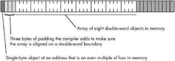
Figure 7-3: Adding padding bytes before an array
On those machines that do not support byte-addressable memory, those compilers that attempt to place the first element of an array on an easily accessed boundary will allocate storage for an array on whatever boundary the machine supports. If the size of each array element is less than the minimum size memory object the CPU supports, the compiler implementer has two options:
-
Allocate the smallest accessible memory object for each element of the array
-
Pack multiple array elements into a single memory cell
The first option has the advantage of being fast, but it wastes memory because each array element carries along some extra storage that it doesn't need. The second option is compact, but it requires extra instructions to pack and unpack data when accessing array elements, which means that accessing elements is slower. Compilers on such machines often provide an option that lets you specify whether you want the data packed or unpacked so you can make the choice between space and speed.
If you're working on a byte-addressable machine (like the 80x86) then you probably don't have to worry about this issue. However, if you're using a high-level language and your code might wind up running on a different machine at some point in the future, you should choose an array organization that is efficient on all machines.
7.2.3 Accessing Elements of an Array
If you allocate all the storage for an array in contiguous memory locations, and the first index of the array is zero, then accessing an element of a one-dimensional array is simple. You can compute the address of any given element of an array using the following formula:
Element_Address = Base_Address + index * Element_Size
The Element_Size item is the number of bytes that each array element occupies. Thus, if the array contains elements of type byte, the Element_Size field is one and the computation is very simple. If each element of the array is a word (or another two-byte type) then Element_Size is two. And so on.
Consider the following Pascal array declaration:
var SixteenInts : array[ 0..15] of integer;
To access an element of the SixteenInts on a byte-addressable machine, assuming 4-byte integers, you'd use this calculation:
Element_Address = AddressOf( SixteenInts) + index*4
In assembly language (where you would actually have to do this calculation manually rather than having the compiler do the work for you), you'd use code like the following to access array element SixteenInts[index] :
mov( index, ebx ); mov( SixteenInts[ ebx*4 ], eax );
7.2.4 Multidimensional Arrays
Most CPUs can easily handle one-dimensional arrays. Unfortunately, there is no magic addressing mode that lets you easily access elements of multidimensional arrays. That's going to take some work and several machine instructions.
Before discussing how to declare or access multidimensional arrays, it would be a good idea to look at how to implement them in memory. The first problem is to figure out how to store a multidimensional object in a one-dimensional memory space.
Consider for a moment a Pascal array of the following form:
A:array[0..3,0..3] of char;
This array contains 16 bytes organized as four rows of four characters . Somehow you have to draw a correspondence between each of the 16 bytes in this array and each of the 16 contiguous bytes in main memory. Figure 7-4 shows one way to do this.
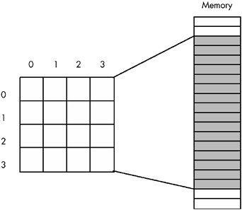
Figure 7-4: Mapping a 4x4 array to sequential memory locations
The actual mapping is not important as long as two things occur:
-
No two entries in the array occupy the same memory location(s)
-
Each element in the array always maps to the same memory location
Therefore, what you really need is a function with two input parameters - one for a row and one for a column value - that produces an offset into a contiguous block of 16 memory locations.
Any old function that satisfies these two constraints will work fine. However, what you really want is a mapping function that is efficient to compute at run time and that works for arrays with any number of dimensions and anybounds on those dimensions. While there are a large number of possible functions that fit this bill, there are two functions that most high-level languages use: row-major ordering and column-major ordering.
7.2.4.1 Row-Major Ordering
Row-major ordering assigns array elements to successive memory locations by moving across the rows and then down the columns . Figure 7-5 demonstrates this mapping.
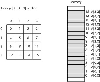
Figure 7-5: Row-major array element ordering
Row-major ordering is the method employed by most high-level programming languages including Pascal, C/C++, Java, Ada, and Modula-2. It is very easy to implement and is easy to use in machine language. The conversion from a two-dimensional structure to a linear sequence is very intuitive. Figure 7-6 on the next page provides another view of the ordering of a 4 —4 array.
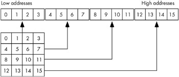
Figure 7-6: Another view of row-major ordering for a 4 —4 array
The actual function that converts the set of multidimensional array indexes into a single offset is a slight modification of the formula for computing the address of an element of a one-dimensional array. The formula to compute the offset for a 4 —4 two-dimensional row-major ordered array given an access of this form:
A[ colindex][ rowindex ]
. . is as follows:
Element_Address = Base_Address + (colindex * row_size + rowindex) * Element_Size
As usual, Base_Address is the address of the first element of the array ( A[0][0] in this case) and Element_Size is the size of an individual element of the array, in bytes. Row_size is the number of elements in one row of the array (four, in this case, because each row has four elements). Assuming Element_Size is one, this formula computes the following offsets from the base address:
| Column Index | Row Index | Offset into Array |
|---|---|---|
|
|
|
|
|
| 1 | 1 |
|
| 2 | 2 |
|
| 3 | 3 |
| 1 |
| 4 |
| 1 | 1 | 5 |
| 1 | 2 | 6 |
| 1 | 3 | 7 |
| 2 |
| 8 |
| 2 | 1 | 9 |
| 2 | 2 | 10 |
| 2 | 3 | 11 |
| 3 |
| 12 |
| 3 | 1 | 13 |
| 3 | 2 | 14 |
| 3 | 3 | 15 |
For a three-dimensional array, the formula to compute the offset into memory is only slightly more complex. Consider a C/C++ array declaration given as follows:
someType A[depth_size][col_size][row_size];
If you have an array access similar to A[depth_index][col_index][row_index] then the computation that yields the offset into memory is the following:
Address = Base + ((depth_index * col_size + col_index)*row_size + row_index) * Element_Size Element_size is the size, in bytes, of a single array element.
For a four-dimensional array, declared in C/C++ as:
type A[bounds0][bounds1][bounds2][bounds3];
. . the formula for computing the address of an array element when accessing element A[i][j][k][m] is as follows:
Address = Base + (((i * bounds1 + j) * bounds2 + k) * bounds3 + m) * Element_Size
If you've got an n -dimensional array declared in C/C++ as follows:
dataType A[b n-1 ][b n-2 ]...[b ];
. . and you wish to access the following element of this array:
A[a n-1 ][a n-2 ]...[a 1 ][a ]
. . then you can compute the address of a particular array element using the following algorithm:
Address := a n-1 for i := n-2 downto 0 do Address := Address * b i + a i Address := Base_Address + Address*Element_Size
7.2.4.2 Column-Major Ordering
Column-major ordering is the other common array element address function. FORTRAN and various dialects of BASIC (such as older versions of Microsoft BASIC) use this scheme to index arrays. Pictorially, a column-major ordered array is organized as shown in Figure 7-7.
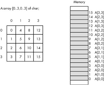
Figure 7-7: Column-major array element ordering
The formula for computing the address of an array element when using column-major ordering is very similar to that for row-major ordering. The difference is that you reverse the order of the index and size variables in the computation. That is, rather than working from the leftmost index to the rightmost, you operate on the indexes from the rightmost towards the leftmost.
For a two-dimensional column-major array, the formula is as follows:
Element_Address = Base_Address + (rowindex * col_size + colindex) * Element_Size
The formula for a three-dimensional column-major array is the following:
Element_Address = Base_Address + ((rowindex*col_size+colindex) * depth_size + depthindex) * Element_Size
And so on. Other than using these new formulas, accessing elements of an array using column-major ordering is identical to accessing arrays using row-major ordering.
7.2.4.3 Declaring Multidimensional Arrays
If you have an m — n array, it will have m — n elements and will require m — n — Element_Size bytes of storage. To allocate storage for an array you must reserve this amount of memory. With one-dimensional arrays, the syntax that the different high-level languages employ is very similar. However, their syntax starts to diverge when you consider multidimensional arrays.
In C, C++, and Java, you use the following syntax to declare a multidimensional array:
data_type array_name [dim 1 ][dim 2 ] . . . [dim n ];
Here is a concrete example of a three-dimensional array declaration in C/C++:
int threeDInts[ 4 ][ 2 ][ 8 ];
This example creates an array with 64 elements organized with a depth of four by two rows by eight columns. Assuming each int object requires 4 bytes, this array consumes 256 bytes of storage.
Pascal's syntax actually supports two equivalent ways of declaring multidimensional arrays. The following example demonstrates both of these forms:
var threeDInts : array[0..3] of array[0..1] of array[0..7] of integer; threeDInts2 : array[0..3, 0..1, 0..7] of integer;
Semantically, there are only two major differences that exist among different languages. The first difference is whether the array declaration specifies the overall size of each array dimension or whether it specifies the upper and lower bounds. The second difference is whether the starting index is zero, one, or a user -specified value.
7.2.4.4 Accessing Elements of a Multidimensional Array
Accessing an element of a multidimensional array in a high-level language isso easy that a typical programmer will do so without considering the associated cost. In this section, we'll look at some of the assembly language sequences you'll need to access elements of a multidimension array to give you a clearer picture of these costs.
Consider again, the C/C++ declaration of the ThreeDInts array from the previous section:
int threeDInts[ 4 ][ 2 ][ 8 ];
In C/C++, if you wanted to set element [i][j][k] of this array to the value of n , you'd probably use a statement similar to the following:
ThreeDInts[i][j][k] = n;
This statement, however, hides a great deal of complexity. Recall the formula needed to access an element of a three-dimensional array:
Element_Address = Base_Address + ((rowindex * col_size + colindex) * depth_size + depthindex) * Element_Size
The ThreeDInts example does not avoid this calculation, it only hides it from you. The machine code that the C/C++ compiler generates is similar to the following:
intmul( 2, i, ebx ); // EBX = 2 * i add( j, ebx ); // EBX = 2 * i + j intmul( 8, ebx ); // EBX = (2 * i + j) * 8 add( k, ebx ); // EBX = (2 * i + j) * 8 + k mov( n, eax ); mov( eax, ThreeDInts[ebx*4] ); // ThreeDInts[i][j][k] = n
Actually, ThreeDInts is special. The sizes of all the array dimensions are nice powers of two. This means that the CPU can use shifts instead of multiplication instructions to multiply EBX by two and by four in this example. Because shifts are often faster than multiplication, a decent C/C++ compiler will generate the following code:
mov( i, ebx ); shl( 1, ebx ); // EBX = 2 * i add( j, ebx ); // EBX = 2 * i + j shl( 3, ebx ); // EBX = (2 * i + j) * 8 add( k, ebx ); // EBX = (2 * i + j) * 8 + k mov( n, eax ); mov( eax, ThreeDInts[ebx*4] ); // ThreeDInts[i][j][k] = n
Note that a compiler can only use this faster code if an array dimension is a power of two. This is the reason many programmers attempt to declare arrays whose dimension sizes are some power of two. Of course, if you must declare extra elements in the array to achieve this goal, you may wind up wasting space ( especially with higher-dimensional arrays) to achieve a small increase in speed.
For example, if you need a 10 —10 array and you're using row-major ordering, you could create a 10 —16 array to allow the use of a shift (by four) instruction rather than a multiply (by 10) instruction. When using column-major ordering, you'd probably want to declare a 16 —10 array to achieve the same effect, since row-major calculation doesn't use the size of the first dimension when calculating an offset into an array, and column-major calculation doesn't use the size of the second dimension when calculating an offset. In either case, however, the array would wind up having 160 elements instead of 100 elements. Only you can decide if this extra space is worth the small increase in speed you'll gain.
[1] Many Pascal compilers provide an option to turn off this array index range checking once your program is fully tested . Turning off the bounds checking improves the efficiency of the resulting program.
[2] BASIC allows you to use floating-point values as array indexes because the original BASIC language did not provide support for integer expressions; it only provided real values and string values.
EAN: 2147483647
Pages: 144