SQL functions
3.7 SQL functions
In this section, we will take a look at various SQL functions in Oracle.
3.7.1 Functions for aggregation
OLAP applications often involve aggregating data across several dimensions. To facilitate these operations, Oracle provides several aggregation capabilities. In addition to the traditional SQL GROUP BY clause, Oracle provides the CUBE, ROLLUP, and GROUPING SETS functions.
The CUBE and ROLLUP operators have been present since Oracle 8i, and the GROUPING SETS operator was introduced in Oracle 9i. The ROLLUP operator is used to compute subtotals along a dimension, and the CUBE operator is used to compute all possible aggregations for a set of GROUP BY columns. The GROUPING SETS operator enables a user to compute multiple independent groupings in one query. In the past, these types of operations were done using report-writing tools. By executing them within the database, they can be executed in parallel and benefit from the various features and query optimizations discussed earlier.
CUBE, ROLLUP, and GROUPING SETS can be used with all the supported aggregates in Oracle, such as COUNT, AVG, MIN, MAX, STDDEV, and VARIANCE and also with the analytical functions discussed in section 3.7.2.
We will now take a detailed look at these functions.
CUBE
The CUBE operator computes aggregates for all possible combinations of the columns in the GROUP BY clause. In the following example, we are computing the CUBE operation for total sales of products by product category and purchase date.
SELECT p.category, t.time_key, SUM(f.purchase_price) FROM product p, purchases f, time t WHERE p.product_id = f.product_id AND t.time_key = f.time_key GROUP BY CUBE (p.category, t.time_key);
The answer to this query (shown below) includes SUM(f.purchase_ price) grouped by (category, time_key), by (category), by (time_key), and a grand total. We have highlighted with arrows the first row in each group.
CATEGORY TIME_KEY SALES ---------- --------------- ---------- ELEC 01-JAN-02 1574137.45 <- (category, time_key) ELEC 02-JAN-02 56.02 ELEC 01-FEB-02 56.02 ELEC 02-FEB-02 1574137.45 HDRW 01-JAN-02 16704.22 HDRW 02-FEB-02 16704.22 MUSC 01-JAN-02 17989.16 MUSC 02-FEB-02 17989.16 ELEC 3148386.94 <- (category) HDRW 33408.44 MUSC 35978.32 01-JAN-02 1608830.83 <- (time_key) 02-JAN-02 56.02 01-FEB-02 56.02 02-FEB-02 1608830.83 3217773.7 <- grand total
ROLLUP
The ROLLUP function creates subtotals, rolling data up from a lower level to a higher level. It also produces a grand, or final, total. The ROLLUP operator is useful for totaling data across a hierarchical dimension such as time.
Referring to the following example, the ROLLUP operation computes the total sales for the groupings (category, time_key), (category), and grand total. We have highlighted the first row of each grouping with arrows.
SELECT p.category, t.time_key, SUM(f.purchase_price) FROM product p, purchases f, time t WHERE p.product_id = f.product_id AND t.time_key = f.time_key GROUP BY ROLLUP (p.category, t.time_key); CATEGORY TIME_KEY SALES ---------- --------------- ---------- ELEC 01-JAN-02 1574137.45 <- (category, time_key) ELEC 02-JAN-02 56.02 ELEC 01-FEB-02 56.02 ELEC 02-FEB-02 1574137.45 HDRW 01-JAN-02 16704.22 HDRW 02-FEB-02 16704.22 MUSC 01-JAN-02 17989.16 MUSC 02-FEB-02 17989.16 HDRW 33408.44 <- (category) ELEC 3148386.94 MUSC 35978.32 3217773.7 <- grand total
In a ROLLUP, the groupings are determined by repeatedly aggregating over the rightmost column in the previous grouping. In the previous example, we first group by (category, time_key) and then by (category). So, to ROLLUP along a hierarchy correctly, we must order the columns from the highest to the lowest level of the hierarchy from left to right. For instance, to ROLLUP along a time hierarchy the column ordering would be (year, month, day).
If we compare the output of the CUBE and ROLLUP, you will notice that ROLLUP only computes some of the possible combinations of groupings in a CUBE. In the previous example, the grouping (time_key) is present in the CUBE but not in the ROLLUP output. The output of a CUBE always includes the output of a ROLLUP.
As the number of columns increases, the CUBE operator can consume a lot of time and space. The number of groupings for a CUBE with two columns is four; with three columns, eight; and so on. The ROLLUP is a much simpler and hence more efficient operation—for two columns, a ROLLUP produces three groupings; for three columns, four; and so on.
GROUPING SETS
Summary tables or materialized views are often used to store precomputed aggregations. If we were to store the result of a CUBE operator, computing all possible combinations of grouping columns, the space requirements could get too large. It is not uncommon for the output of a CUBE to be several times larger than the size of the tables themselves! This problem is overcome by using GROUPING SETS, which provide the capability to selectively compute only interesting combinations of groupings instead of the entire CUBE.
In the following example, we calculate sales by (category, time_key), by (category, state_id), by (time_key, region), and the grand total of sales, denoted by (). We choose not to calculate other combinations such as detailed sales for each category, time_key, and state.
SELECT p.category as cat, t.time_key, g.region, g.state_id as st, SUM(f.purchase_price) sales FROM product p, purchases f, time t, geography g WHERE p.product_id = f.product_id AND t.time_key = f.time_key AND g.state_id = f.state_id GROUP BY GROUPING SETS ((p.category, t.time_key), (p.category, g.state_id), (t.time_key, g.region), ()); CAT TIME_KEY REGION ST SALES ---- --------- --------- -- --------- ELEC 01-JAN-02 1574137.45 <- (category,time_key) ELEC 02-JAN-02 56.02 ELEC 01-FEB-02 56.02 ELEC 02-FEB-02 1574137.45 HDRW 01-JAN-02 16704.22 HDRW 02-FEB-02 16704.22 MUSC 01-JAN-02 17989.16 MUSC 02-FEB-02 17989.16 ELEC CA 1574193.47 <- (category,state_id) ELEC MA 1484355.05 ELEC NH 89838.42 HDRW CA 13115.79 HDRW NH 16704.22 HDRW WI 3588.43 MUSC CA 2977.3 MUSC NH 7192.53 MUSC OH 7819.33 MUSC WI 17989.16 01-JAN-02 West 2977.3 <- (time_key,region) 01-JAN-02 MidWest 7819.33 01-JAN-02 NorthEast 1598034.2 02-JAN-02 NorthEast 56.02 01-FEB-02 West 56.02 02-FEB-02 West 1587253.24 02-FEB-02 MidWest 21577.59 3217773.7 <- grand total
Note that ROLLUP is a special case of a GROUPING SET. ROLLUP(category, time_key) is equivalent to GROUPING SETS ((category, time_key), (category), ()).
You may specify multiple GROUPING SETS in a query. This offers a concise way to specify a cross-product of groupings across multiple dimensions. Suppose we would like to compute sales by product category on the geography dimension for the (state, city) columns and for the time dimension for the (year, quarter) columns. Instead of specifying all combinations involving these four columns, we could simply use the following query. This is known as concatenated GROUPING SETS.
SELECT p.category as cat, t.quarter as quart, t.year, g.state_id as st, g.region, SUM(f.purchase_price) sales FROM purchases f, time t, geography g, product p WHERE p.product_id = f.product_id AND t.time_key = f.time_key AND g.state_id = f.state_id GROUP BY p.category, GROUPING SETS (g.state_id, g.region), GROUPING SETS (t.quarter, t.year); CAT QUART YEAR ST REGION SALES ---- ----- ----- -- ---------- ---------- ELEC 1 CA 1574193.47 <- (quarter,state) ELEC 1 MA 1484355.05 ELEC 1 NH 89838.42 ... MUSC 1 WI 17989.16 ELEC 1 West 1574193.47 <- (quarter,region) ELEC 1 NorthEast 1574193.47 ... MUSC 1 NorthEast 7192.53 ELEC 2002 CA 1574193.47 <- (year, state) ELEC 2002 MA 1484355.05 ELEC 2002 NH 89838.42 ... MUSC 2002 WI 17989.16 ELEC 2002 West 1574193.47 <- (year, region) ELEC 2002 NorthEast 1574193.47 ... MUSC 2002 NorthEast 7192.53
The p.category column that is outside the GROUPING SETS is present in all the groupings. Thus, the previous query computes the four groupings: (category, quarter, state), (category, quarter, region), (category, year, state), and (category, year, region).
GROUPING and GROUPING_ID functions
The CUBE, ROLLUP, and GROUPING SETS operators all compute multiple levels of aggregations in one query. Your application may need a way to identify the portion of the output corresponding to a particular level of aggregation. The SQL functions, GROUPING() and GR OUPING_ID() provide a mechanism to identify which rows in the answer correspond to which level of aggregation.
The following query illustrates the behavior of the GROUPING() function.
SELECT p.category as cat, t.time_key, SUM(f.purchase_price) sales, GROUPING(p.category) grp_c, GROUPING(t.time_key) grp_t FROM product p, purchases f, time t WHERE p.product_id = f.product_id AND t.time_key = f.time_key GROUP BY ROLLUP (p.category, t.time_key); CAT TIME_KEY SALES GRP_C GRP_T ---- --------- ---------- ----- ----- ELEC 01-JAN-02 1574137.45 0 0 <- (category,time_key) ELEC 02-JAN-02 56.02 0 0 ELEC 01-FEB-02 56.02 0 0 ELEC 02-FEB-02 1574137.45 0 0 HDRW 01-JAN-02 16704.22 0 0 HDRW 02-FEB-02 16704.22 0 0 MUSC 01-JAN-02 17989.16 0 0 MUSC 02-FEB-02 17989.16 0 0 HDRW 4455.58 0 0 * ELEC 3148386.94 0 1 <- (category) HDRW 37864.02 0 1 * MUSC 35978.32 0 1 3222229.28 1 1 <- grand total
For each grouping, the GROUPING(category) returns a value of 0 if the category column is in the group and 1 otherwise. Similarly, GROUPING(time_key) returns a value of 0 if the time_key column is in the group and 1 otherwise. Thus, each level of aggregation can be identified from the values of the GROUPING() function. The group (category, time_key) has GROUPING function values (0,0); the group (category) has GROUPING function values (0,1). Note that the grand total row can be easily identified as the row where each grouping function column has the value of 1.
In the output of CUBE or ROLLUP, the rows that correspond to a higher level of aggregation have the value NULL for the columns that have been aggregated away. Another use of the GROUPING() function is to distinguish this NULL from actual NULL values in the data. For example, look carefully at the rows in the previous output marked with an asterisk. Both these rows have a NULL value in the time_key column. The first of these corresponds to rows in the purchases table for the HDRW category, where the time_key value was unavailable (NULL). In the second one, we have aggregated away the time_key values and hence this row corresponds to aggregation at the category level. The GROUPING() function distinguishes these two similar-looking rows. For the first case, the GROUPING(time_key) is 0; in the second, it is 1.
Instead of using GROUPING() for each column, you can use GROUPING_ID() with all the columns together, as follows:
SELECT p.category, t.time_key, SUM(f.purchase_price), GROUPING_ID(p.category,t.time_key) gid FROM product p, purchases f, time t WHERE p.product_id = f.product_id AND t.time_key = f.time_key GROUP BY ROLLUP (p.category, t.time_key); CATEGORY TIME_KEY SALES GID -------- --------- ---------- ---------- ELEC 01-JAN-02 1574137.45 0 <- (category, time_key) ELEC 02-JAN-02 56.02 0 ELEC 01-FEB-02 56.02 0 ELEC 02-FEB-02 1574137.45 0 HDRW 01-JAN-02 16704.22 0 HDRW 02-FEB-02 16704.22 0 MUSC 01-JAN-02 17989.16 0 MUSC 02-FEB-02 17989.16 0 HDRW 4455.58 0 ELEC 3148386.94 1 <- (category) HDRW 37864.02 1 MUSC 35978.32 1 3222229.28 3 <- grand total
If you consider all the individual GROUPING() functions together as a binary number, GROUPING_ID() returns the corresponding decimal number. Thus, in the previous example, if GROUPING(p.category) is 0 and GROUPING(t.time_key) is 1, then GROUPING_ID(p.category, t.time_key) is the binary number formed by 01, which is the decimal number 1. For the grand total row, GROUPING(p.category) is 1 and GROUPING(t.time_key) is 1, and, hence, the GROUPING_ID(p.category, t.time_key) is the binary number 11, which is the number 3. The GROUPING_ID() is thus a much more compact representation than individual grouping functions but is not as straightforward to interpret as separate GROUPING() functions on each column.
3.7.2 SQL functions for analytical computing
Decision support applications often need to answer questions such as: What were the top-ten selling products in 2001? or How do the regional sales for January this year compare against last year's sales? or What are the cumulative sales numbers for each month this year?
Though these questions sound quite simple, the traditional SQL queries needed to answer these questions can be extremely complex. These queries are quite hard to optimize and may require multiple scans over the data. They may perform poorly or may require application layer processing. Hence, many database vendors started an initiative to provide SQL extensions to concisely represent these types of queries. The extensions are now part of the SQL99 standard. By using the analytical functions in the database, these calculations can take advantage of parallelism and other optimization techniques in the database.
The analytical functions in Oracle provide many useful capabilities, including the following:
-
Ranking functions can be used to answer queries for top-N items. They can also be used to classify data into buckets. Examples of ranking functions include RANK(), DENSE_RANK(), and NTILE(). You can also compute the rank of a quantity as if it were hypothetically inserted into the data.
-
Moving window functions can be used to calculate quantities such as cumulative sum or moving average. Moving window calculations are very useful when dealing with data over a period of time. For instance, if you want to know the average sales of a product over the past seven days, six months, five years, and so on.
-
Reporting aggregates can be used to see the aggregate value side by side with the detailed rows that contributed to it. For instance, if you want to compare sales of each product with the average sales of all products.
-
Lag and lead functions can be used to do period-over-period comparisons—for example, comparing sales of one year with the previous.
-
Statistical functions, such as linear regression, and advanced aggregate functions, such as covariance, can be used to do trend analysis.
We will now look at these functions in detail with examples.
Ranking functions
Ranking functions rank the rows in a data set after ordering it by a specified criterion. The following SQL example answers the query: What were the top-selling ten products? In this case, the ordering criterion is the total sales for the product, as specified by the ORDER BY clause.
SELECT * FROM (SELECT p.product_id, SUM(f.purchase_price) as sales, RANK() over (ORDER BY SUM(f.purchase_price)) as rank FROM purchases f, product p WHERE f.product_id = p.product_id GROUP BY p.product_id) WHERE rank <= 10; PRODUCT_ID SALES RANK ---------- ---------- --------- SP1222 38832.31 1 SP1244 39145.54 2 SP1256 39354.24 3 SP1263 39458.78 4 SP1236 39699.14 5 SP1220 39893.6 6 SP1231 40080.61 7 SP1242 40208.33 8 SP1248 40312.98 9 SP1254 40418.02 10
This query has two parts—an inner query that computes the RANK() function and the outer one that selects the top ten of these ranks. The inner query computes the aggregate function SUM(f.purchase_price) for each product_id. It then orders the result by the sales and applies the RANK() function to it. The RANK() function assigns ranks from 1 to N, skipping ranks in case of ties. Thus, if there were two products with the same sales, with rank 3, the next rank would be 5. A variant of RANK() is the DENSE_RANK() function which assigns contiguous ranks despite ties. For instance, if two products had the same rank, 3, DENSE_RANK() would assign the next rank to be 4.
The ORDER BY clause further specifies ascending versus descending order and whether to consider NULL values as first or last in the order. The default order is ascending. NULLS LAST is the default for ascending order and NULLS FIRST for descending order. In the following query, the ORDER BY is in descending order and NULL values are to be considered last in the order.
SELECT p.product_id, SUM(f.purchase_price) as sales, RANK() over (ORDER BY SUM(f.purchase_price) DESC NULLS LAST) as rank FROM purchases f, product p WHERE f.product_id = p.product_id GROUP BY p.product_id; PRODUCT_ SALES RANK -------- ---------- ---------- SP1046 1115634.20 1 SP1056 1109091.08 2 SP1036 1107147.52 3 SP1060 1095253.99 4 SP1042 1002747.91 5 SP1051 979279.86 6 SP1041 941985.49 7 SP1054 919424.74 8 SP1048 919051.12 9 SP1052 853124.58 10 SP1222 81385.09 161 SP1039 162 <- nulls last
It is important to note that analytical functions are applied after the WHERE, GROUP BY, and HAVING clauses of the query are computed. So aggregate functions such as SUM(f.purchase_price) are available as ordering criteria to the ranking function.
PARTITION BY clause
A useful feature with analytic functions is that you can divide the data into groups and then apply the function to each group. The group is specified using the PARTITION BY clause. For instance, if you wanted to rank the products in each product category, we could use the following query. (Only five ranks are shown in each category for lack of space.)
SELECT p.category, p.product_id, SUM(f.purchase_price) as sales, RANK() over (PARTITION BY p.category ORDER BY SUM(f.purchase_price)) as rank FROM purchases f, product p WHERE f.product_id = p.product_id GROUP BY p.category, p.product_id; CATEGORY PRODUCT_ID SALES RANK ---------- ---------- ---------- ---------- ELEC SP1080 40495.3 1 ELEC SP1073 41440.34 2 ELEC SP1086 41599.05 3 ELEC SP1065 41939.38 4 ELEC SP1084 42253.72 5 ... HDRW SP1222 38832.31 1 HDRW SP1236 39699.14 2 HDRW SP1220 39893.6 3 HDRW SP1231 40080.61 4 HDRW SP1214 40930.96 5 ...
Figure 3.9 illustrates how the PARTITION BY clause affects the computation of RANK(). As before, the query first computes the sales for each product_id and category. The PARTITION BY clause in the query then divides this result by category. For each category, the RANK() function assigns a rank to the product_ids ordered according to their sales.
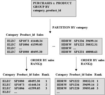
Figure 3.9: PARTITION BY clause.
You can calculate ranks using different PARTITION and ORDER BY expressions in the same query. The PARTITION BY clause used by analytical functions is completely unrelated to the data partitioning feature of Oracle discussed in section 3.3.
Bucketing functions
Analytical applications often require the ability to classify data into buckets or to determine how a given product compares in the entire range of products. The ranking functions CUME_DIST(), PERCENT_RANK(), and NTILE() provide this functionality.
CUME_DIST() calculates the position of a value in relation to a set of values, returning a value between 0 and 1. PERCENT_RANK() gives the rank of a row relative to all the rows in a data set Both CUME_DIST() and PERCENT_RANK() have a value between 0 and 1.
The following examples illustrate the difference between CUME_DIST and PERCENT_RANK functions. (Only rows for the HDRW category are shown.)
SELECT p.category, p.product_id, SUM(f.purchase_price) as sales, CUME_DIST() over (PARTITION BY p.category ORDER BY SUM(f.purchase_price)) as cume_dist FROM purchases f, product p WHERE f.product_id = p.product_id GROUP BY p.category, p.product_id; HAVING SUM(f.purchase_price) < 100000 ; CATE PRODUCT_ SALES CUME_DIST ---- -------- ---------- ---------- ... HDRW SP1222 81385.09 .142857143 HDRW SP1236 82520.97 .285714286 HDRW SP1220 82622 .428571429 HDRW SP1231 83073.57 .571428571 HDRW SP1214 83841.66 .714285714 HDRW SP1212 99663.51 .857142857 HDRW SP1232 99863.42 1 ...
The position of the first row is 1 and there are 7 rows in all, so CUME_ DIST() is 1/7, or 0.142857143, and so on. The PERCENT_RANK() is computed as RANK() of the row - 1, divided by total ranks - 1. Thus, PERCENT_RANK() for the first row is always 0. The RANK() of the second row is 2 and there are 7 ranks, so PERCENT_RANK is 1/6, or 0.166666667.
SELECT p.category, p.product_id, SUM(f.purchase_price) as sales, PERCENT_RANK() over (PARTITION BY p.category ORDER BY SUM(f.purchase_price)) as pct_rank FROM purchases f, product p WHERE f.product_id = p.product_id GROUP BY p.category, p.product_id HAVING SUM(f.purchase_price) < 100000; CATE PRODUCT_ SALES CUME_DIST ---- -------- ---------- ---------- ... HDRW SP1222 81385.09 0 HDRW SP1236 82520.97 .166666667 HDRW SP1220 82622 .333333333 HDRW SP1231 83073.57 .5 HDRW SP1214 83841.66 .666666667 HDRW SP1212 99663.51 .833333333 HDRW SP1232 99863.42 1 ...
The NTILE() function is useful to compute statistical measures such as quartile and percentile. The NTILE(N) function orders the data using specified criteria and then divides the result into N buckets, assigning the bucket number to all rows in each bucket. If N is 100, the quantity is known as the percentile and if N is 4, quartile.
The following query calculates the NTILE(4) in each product category using the sales for each product in the category. NTILE(4) assigns a number between one and four to each row.
SELECT p.category, p.product_id, SUM(f.purchase_price) as sales, NTILE(4) over (PARTITION BY p.category ORDER BY SUM(f.purchase_price)) as quartile FROM purchases f, product p WHERE f.product_id = p.product_id GROUP BY p.category, p.product_id; CATE PRODUCT_ SALES CUME_DIST ---- -------- ---------- ---------- ... HDRW SP1222 81385.09 1 HDRW SP1236 82520.97 1 HDRW SP1220 82622 2 HDRW SP1231 83073.57 2 HDRW SP1214 83841.66 3 HDRW SP1212 99663.51 3 HDRW SP1232 99863.42 4 ...
The buckets generated by the NTILE(4) function all have approximately the same number of rows; however, the range between lowest and highest value in each bucket may differ. This is known as an equi-height histogram. On the other hand, the WIDTH_BUCKET() function can be used to generate equi-width histograms where the data is distributed into buckets such that each bucket has the same range but can have differing numbers of rows.
SELECT p.product_id, SUM(f.purchase_price) as sales, WIDTH_BUCKET(SUM(f.purchase_price), 80000, 120000, 4) as width_bucket FROM purchases f, product p WHERE f.product_id = p.product_id and p.category = 'HDRW' GROUP BY p.product_id ORDER BY sales; PRODUCT_ SALES WIDTH_BUCKET -------- ---------- ------------ SP1222 81385.09 1 SP1236 82520.97 1 SP1220 82622.00 1 SP1231 83073.57 1 SP1214 83841.66 1 SP1212 99663.51 2 SP1232 99863.42 2 SP1224 100825.37 3 SP1234 109433.07 3 SP1219 111809.95 4 SP1239 112749.64 4 SP1213 112749.90 4 ... SP1233 148895.43 5 SP1221 167743.34 5
The inputs to the WIDTH_BUCKET are the end points for the ranges to be considered and the number of intermediate points. The function then divides the range of sales into the equi-width buckets by placing equally spaced points in between the end points and assigns each row to buckets according to which range it falls into. In our examples the range from 80000 to 120000 is divided into five approximately equal ranges (or five buckets). We can see that each bucket can have different numbers of rows.
Window aggregate functions
Window aggregate functions let you compute a function such as SUM over a specified window of rows relative to the current row. These functions allow you to do moving window operations such as cumulative sum or moving average.
The following SQL statement answers the query: What are the cumulative sales numbers for each month so far this year? The query first computes the SUM(f.purchase_price) for each month. The expression SUM(SUM(f.purchase_price)) indicates that we are further summing the sales, in this case for all months preceding the current month. The ROWS UNBOUNDED PRECEDING specifies that the window is all rows before and including the current row. A window specified using numbers of rows preceding or following the current row is known as a physical window.
SELECT t.month, SUM(f.purchase_price) as sales, SUM(SUM(f.purchase_price)) OVER (ORDER BY t.month ROWS UNBOUNDED PRECEDING) as cumulative_sales FROM purchases f, time t WHERE f.time_key = t.time_key GROUP BY t.month; MONTH SALES CUMULATIVE_SALES ------ ---------- ---------------- 1 8989096.34 8989096.34 2 17213413.50 26202509.90 3 429035.78 26631545.70 4 4520301.94 31151847.60 5 1268317.48 32420165.10 6 7092585.46 39512750.50 ...
In the next example, we are computing, for each month, the moving average of the sales for that month and the two months preceding it. This is specified by the ROWS 2 PRECEDING clause.
SELECT t.month, SUM(f.purchase_price) as sales, AVG(SUM(f.purchase_price)) OVER (ORDER BY t.month ROWS 2 PRECEDING) as moving_average FROM purchases f, time t WHERE f.time_key = t.time_key GROUP BY t.month; MONTH SALES MOVING_AVERAGE ---------- ---------- -------------- 1 8989096.34 8989096.34 2 17213413.5 13101254.90 3 429035.78 8877181.89 4 4520301.94 7387583.75 5 1268317.48 2072551.73 6 7092585.46 4293734.96 ...
If, instead, we wanted the window to include the current month and two months following it, the window expression would simply change to ROWS 2 FOLLOWING. A physical window is good only if you have dense data—for instance, if you have gaps in your dates, a physical window may not be very meaningful.
Instead of specifying the offset using rows, you can specify a logical window using an interval of values around the current value. For instance, if the ordering expression is of DATE type, you can specify a logical window using a constant expression or an INTERVAL DAY, MONTH, or YEAR expression. Logical windows are only allowed for numeric, date, or interval data types. The following example shows sales being computed over a five day interval including two days before and after the current date. In our example, the interval for the dates 2-Apr-02 consists of dates from 31-Mar-02 through 4-Apr-02, and that for 7-Jul-02 consists of dates from 5-Jul-02 through 8-Jul-02, as shown in the answer.
SELECT t.time_key, SUM(f.purchase_price) as sales, SUM(SUM(f.purchase_price)) OVER (ORDER BY t.time_key RANGE BETWEEN INTERVAL '2' DAY PRECEDING AND INTERVAL '2' DAY FOLLOWING) as sales_5_day FROM purchases f, time t WHERE f.time_key = t.time_key GROUP BY t.time_key; TIME_KEY SALES SALES_5_DAY --------- ---------- ----------- 01-JAN-02 8989040.32 8989096.34 02-JAN-02 56.02 8989096.34 01-FEB-02 3401896.62 17213525.6 02-FEB-02 13811629 17213525.6 02-MAR-02 429035.78 429035.78 30-MAR-02 448.19 1958695.44 _ 31-MAR-02 448.19 1960040.01 | 01-APR-02 1957799.06 1960936.39 | 02-APR-02 1344.57 1962280.96 <- current row | logical 03-APR-02 896.38 1961832.77 | interval 04-APR-02 1792.76 4033.71 _| 08-APR-02 2562502.88 2562502.88 06-MAY-02 839281.7 1268317.48 07-MAY-02 429035.78 1268317.48 01-JUN-02 6192443.48 7092585.46 03-JUN-02 900141.98 7092585.46 02-JUL-02 56.02 56.02 _ 05-JUL-02 2240.95 2268.96 | 07-JUL-02 28.01 2296.97 <- current row | logical 08-JUL-02 28.01 56.02 _| interval
The previous example used the BETWEEN clause to specify upper and lower bounds for the interval. This can also be used with a physical offset (e.g., ROWS BETWEEN 2 PRECEDING AND 2 FOLLOWING).
Reporting aggregates
Suppose we want to answer the question: What is the best-selling product category for each sales region? If we try to write a SQL query for this, we will quickly find that the SQL required to answer such a simple question is very complex. For example, one way of doing it would be to first create a table, say total_sales, with the total sales by product category for each sales region. Then further aggregate this table to find the maximum sales for each region, stored in tables, max_sales. Then join the total_sales table to the max_sales table to find those rows that correspond to the maximum sales for each region and return the corresponding product categories. You could also write all these steps in one big SQL query involving several subqueries, but it is quite cumbersome.
The reason why these types of questions are so complex is that when you ask for a simple aggregate such as SUM or MAX in SQL, you lose the individual rows contributing to the aggregate. You only get one row back, which is the aggregate. So when we computed the maximum sales in the max_sales table, we lost knowledge about the individual product categories that had this value of sales.
Reporting aggregates solve this problem by reporting the computed aggregate value side by side with all the detail rows that contributed to it. As with other analytical functions, you can use the PARTITION BY clauses to divide the data before computing the reporting aggregate.
The following query finds the maximum sales for each region, using a reporting aggregate. The PARTITION BY clause simply divides the data by region. The reporting aggregate MAX(SUM(f.purchase_price)) computes the maximum of sales for each region and reports it for each product category value. Thus, the value of max_sales for the region is repeated for each product category in each region. The way we identify that it is a reporting aggregate and not a regular aggregate is the OVER clause.
SELECT p.category, g.region, SUM(f.purchase_price) as regional_prod_sales, MAX(SUM(f.purchase_price)) OVER (PARTITION BY g.region) as max_sales FROM product p, geography g, purchases f WHERE f.product_id = p.product_id AND f.state_id = g.state_id GROUP BY p.category, g.region; CATEGORY REGION REGIONAL_PROD_SALES MAX_SALES ---------- ---------- ------------------- ---------- HDRW MidWest 8044.01 25808.49 MUSC MidWest 25808.49 25808.49 * ELEC NorthEast 1574193.47 1574193.47 * HDRW NorthEast 16704.22 1574193.47 MUSC NorthEast 7192.53 1574193.47 ELEC West 1574193.47 1574193.47 * HDRW West 13115.79 1574193.47 MUSC West 2977.3 1574193.47
Now to answer our original question: What is the best-selling product category for each sales region? All we need to do is select those rows from the previous answer where the regional_prod_sales is the same as the max_ sales. These rows are marked with an asterisk in the preceding output.
SELECT category, region, regional_prod_sales FROM ( SELECT p.category, g.region, SUM(f.purchase_price) as regional_prod_sales, MAX(SUM(f.purchase_price)) OVER (PARTITION BY g.region) as max_sales FROM product p, geography g, purchases f WHERE f.product_id = p.product_id AND f.state_id = g.state_id GROUP BY p.category, g.region ) WHERE regional_prod_sales = max_sales; CATEGORY REGION REGIONAL_PROD_SALES MAX_SALES ---------- ---------- ------------------- ---------- MUSC MidWest 25808.49 25808.49 ELEC NorthEast 1574193.47 1574193.47 ELEC West 1574193.47 1574193.47
Another example where reporting aggregates come in handy is to report the salary of each employee along with the average salary in the department.
SELECT employee, department, salary AVG(salary) OVER (PARTITION by department) as avg_dept_salary FROM payroll;
A special case of a reporting aggregate is the RATIO_TO_REPORT function, which computes the ratio of a value in a set to the sum of the values in that set. The following example finds the ratio of the sales in each product category to the total sales for all product categories. SUM(SUM(f.purchase_price)) computes the total sales for each product category. RATIO_TO_REPORT is essentially a short form for dividing reg_sales/reg_sales_total.
SELECT category, SUM(f.purchase_price) reg_sales, SUM(SUM(f.purchase_price)) OVER () as reg_sales_total, RATIO_TO_REPORT(SUM(f.purchase_price)) OVER () as ratio_to_report FROM product p, purchases f WHERE f.product_id = p.product_id GROUP BY p.category; CATE REG_SALES REG_SALES_TOTAL RATIO_TO_REPORT ---- ----------- --------------- --------------- ELEC 33334833.10 39520369.7 .843484848 HDRW 2962332.61 39520369.7 .074957108 MUSC 3223204.06 39520369.7 .081558044
An interesting aspect of the previous example is that it uses an empty OVER() clause. This simply means that the function is being computed without any partition by clause (i.e., over all rows).
Lag and lead functions
Lag and lead functions provide access to values of a column from a row at a known offset from the current row. For instance, Lag(sales, 1) gives the value of the sales column in the previous row. Lead(sales, 1) gives the value of the sales column in the next row. Thus, queries that would otherwise need to join a table to itself can be done without the join. For instance, the following query reports the sales by month alongside the sales for the previous month and the following month for the year 2002.
SELECT t.month, SUM(f.purchase_price) as sales, LAG(SUM(f.purchase_price),1) OVER (ORDER BY t.month) as sales_last_month, LEAD(SUM(f.purchase_price),1) OVER (ORDER BY t.month) as sales_next_month FROM purchases f, time t WHERE f.time_key = t.time_key AND t.year = 2002 GROUP BY t.month; MONTH SALES SALES_LAST_MONTH SALES_NEXT_MONTH ---------- ---------- ----------------- ---------------- 1 8989096.34 17213413.5 2 17213413.5 8989096.34 429035.78 3 429035.78 17213413.5 4520301.94 4 4520301.94 429035.78 1268317.48 5 1268317.48 4520301.94 7092585.46 6 7092585.46 1268317.48 ...
Lag and lead could be used to do period over period comparisons of sales. For instance, to compare sales for a quarter to the same quarter a year ago (i.e., four quarters ago), you could use LAG(sales, 4).
Note that if the previous (or next) row is not present, Lag (Lead) returns the NULL value.
FIRST and LAST functions
In some situations, you may need to order data by a certain quantity and do analysis based on the first and last items in that order. The FIRST and LAST aggregation functions allow you to do such operations. For instance, the following query finds the number of purchases made for the costliest and cheapest products in each category. It first orders the products in each category by their sell_price and then aggregates the rows obtained using COUNT(*) to find numbers of purchases made for those products that rank FIRST or LAST. Note that the aggregate serves as a tiebreaker if there are several candidates for the FIRST or LAST place by generating one row for all of them.
SELECT p.category cat, SUM(f.purchase_price) total_sales, MIN(p.sell_price) cheap_prod, COUNT(*) KEEP (DENSE_RANK FIRST ORDER BY p.sell_price) cheap_sales, MAX(p.sell_price) costly_prod, COUNT(*) KEEP (DENSE_RANK LAST ORDER BY p.sell_price) costly_sales FROM purchases f, product p WHERE f.product_id = p.product_id GROUP BY p.category; CAT TOTAL_SALES CHEAP_PROD CHEAP_SALES COSTLY_PROD COSTLY_SALES ---- ----------- ---------- ----------- ----------- ------------ ELEC 33327213.9 24.99 16141 1267.89 15036 HDRW 2962332.61 15.67 9980 18 5001 MUSC 3223204.06 10 2305 15.67 13710
FIRST and LAST functions can be used to find sales trends—for instance, in our example we find that in the ELEC category, sales for the costliest items are about the same as for the cheaper ones, whereas in the HDRW category, about a $3 price difference almost cuts the purchases by half.
The FIRST and LAST functions can also be used as reporting aggregates.
Statistical analysis functions
Business decisions may often be influenced by relationships between various quantities. For instance, the price of an item may influence how many items were sold. Linear regression analysis is a statistical technique used to quantify how one quantity affects or determines the value of another. The idea is to fit the data for two quantities along a straight line as accurately as possible. This line is called the regression line. Some of the functions of interest are the slope of the line, y-intercept of the line, and the coefficient of determination (which is how closely the line fits the points). Oracle provides various diagnostic functions commonly used for this analysis, such as standard error and regression sum of squares.
The linear regression functions are all computed simultaneously in a single pass through the data. They can be treated as regular aggregate functions or reporting aggregate functions.
The following example illustrates the use of some of these functions. Here, we are computing the slope, intercept, and coefficient of determination of the regression line for sell_price and purchase_price for products in each product category.
SELECT p.category cat, REGR_SLOPE(p.sell_price, f.purchase_price) slope, REGR_INTERCEPT(p.sell_price, f.purchase_price) intercept, REGR_R2(p.sell_price, f.purchase_price) coeff_determination FROM purchases f, product p WHERE f.product_id = p.product_id GROUP BY p.category; CAT SLOPE INTERCEPT COEFF_DETERMINATION ---- ----------- ---------- ------------------- ELEC .830878246 -87.405372 .831264004 HDRW -.00003465 16.4546582 .000057048 MUSC -.00005981 14.8659674 .000053216
From this analysis, we can see that the relationship between sell_price and purchase_price for the ELEC category can be closely modeled by a straight line. However, for the HDRW and MUSC category, the line is not a very good fit.
To support linear regression analysis, Oracle also provides some new aggregate functions to compute covariance of a population (COVAR_POP) or sample (COVAR_SAMP) and correlation (CORR) between variables.
Inverse percentile
Previously, we mentioned the CUME_DIST() function, which determines the position of each row of data with respect to the entire set. This is also known as a percentile. An inverse percentile performs the reverse operation (i.e., returns the data value that corresponds to a given percentile value in an ordered set of rows).
The following query computes the CUME_DIST() of sales for each category. Here the rows are ordered by SUM(purchase_price), and each row is assigned a value between 0 and 1. We only show some of the rows.
SELECT p.category, p.product_id, SUM(f.purchase_price) as sales, CUME_DIST() over (PARTITION BY p.category ORDER BY SUM(f.purchase_price)) as cume_dist FROM purchases f, product p WHERE f.product_id = p.product_id GROUP BY p.category, p.product_id; CATE PRODUCT SALES CUME_DIST ---- -------- ---------- ---------- ... ELEC SP1100 150155.8 .495412844 ELEC SP1093 150337.4 .504587156 <- PERCENTILE_DISC(0.5) ELEC SP1076 150717.89 .513761468 ... HDRW SP1213 112749.9 .461538462 HDRW SP1217 113019.02 .5 <- PERCENTILE_DISC(0.5) HDRW SP1122 113648.09 .538461538 ... MUSC SP1251 114592.31 .481481481 MUSC SP1253 114840.43 .518518519 <- PERCENTILE_DISC(0.5) MUSC SP1264 115221.38 .555555556 ...
There are two flavors of inverse percentile—PERCENTILE_DISC() assumes that the values are discrete and returns the data value that corresponds to the nearest CUME_DIST() value greater than the percentile specified. PERCENTILE_CONT() assumes that the values are continuous and returns the interpolated value corresponding to the given percentile. In the previous example, the sales value that corresponds to PERCENTILE_ DISC(0.5) for the HDRW category is 113019.02 and for MUSC category is 114840.43.
The following example illustrates the use of the inverse percentile functions. Note that since the PERCENTILE_DISC and PERCENTILE_ CONT functions must return a single data value, an ORDER BY criterion must be specified and must consist of a single expression.
SELECT p.category, p.product_id, SUM(f.purchase_price) as sales, PERCENTILE_DISC(0.5) WITHIN GROUP (ORDER BY SUM(f.purchase_price)) OVER (PARTITION BY p.category) as pct_disc, PERCENTILE_CONT(0.5) WITHIN GROUP (ORDER BY SUM(f.purchase_price)) OVER (PARTITION BY p.category) as pct_cont FROM purchases f, product p WHERE f.product_id = p.product_id GROUP BY p.category, p.product_id; CATE PRODUCT_ SALES PCT_DISC PCT_CONT ---- -------- ---------- ---------- ---------- ... ELEC SP1100 150155.8 150337.4 150337.4 ELEC SP1093 150337.4 150337.4 150337.4 ELEC SP1076 150717.89 150337.4 150337.4 ... HDRW SP1213 112749.9 113019.02 113333.555 HDRW SP1217 113019.02 113019.02 113333.555 HDRW SP1122 113648.09 113019.02 113333.555 ... MUSC SP1251 114592.31 114840.43 114840.43 MUSC SP1253 114840.43 114840.43 114840.43 MUSC SP1264 115221.38 114840.43 114840.43 ...
In this example, PERCENTILE_DISC and PERCENTILE_CONT have been used as reporting aggregates.
What-if analysis
Analytical applications often involve what-if analysis. For instance, you may want to know how a new product will perform relative to other products in its category, given a projected sales figure. Oracle provides a family of hypothetical rank and distribution functions for this purpose. With these functions, you can ask to compute the RANK(), PERCENT_RANK(), or CUME_DIST() of a given value, if it were hypothetically inserted into a set of values.
Hypothetical rank functions take an ordering condition and a constant data value to be inserted into the ordered set. To illustrate we show the sales for different products and then find the rank for a hypothetical product.
The following query shows the sales for different products in the HDRW category and their respective ranks.
SELECT p.product_id, SUM(f.purchase_price) sales, RANK() OVER (ORDER BY SUM(f.purchase_price)) as rank FROM purchases f, product p WHERE f.product_id = p.product_id and p.category = 'HDRW' GROUP BY p.product_id; CATE PRODUCT_ SALES RANK ---- -------- ---------- ----- HDRW SP1222 81385.09 1 HDRW SP1236 82520.97 2 HDRW SP1220 82622 3 HDRW SP1231 83073.57 4 HDRW SP1214 83841.66 5 <- insert hypothetical value 98000.00 HDRW SP1212 99663.51 6 HDRW SP1232 99863.42 7 HDRW SP1224 100825.37 8 ...
Now, suppose we want to find the hypothetical rank of a product with sales of $98,000.00. From the previous output, we can see that this value, if inserted into the data, would get a rank of 6. The following query asks for the hypothetical rank.
SELECT RANK(98000.00) WITHIN GROUP (ORDER BY SUM(f.purchase_price)) as hrank, FROM purchases f, product p WHERE f.product_id = p.product_id and p.category = 'HDRW' GROUP BY p.product_id; HRANK ---------- 6
The way to recognize a hypothetical rank function in a query is the WITHIN GROUP clause and a constant expression within the RANK() function.
3.7.3 User-defined aggregates
Oracle 9i introduced a feature to allow users to define custom aggregate functions. These aggregates can be used like regular aggregates or like analytical functions as reporting aggregates and window aggregates. Userdefined aggregates can be used when there is a complex function that cannot be expressed in SQL or a complex data representation such as objects or LOBs. These are typically useful in financial applications.
User-defined aggregates are part of Oracle's extensibility framework. To define a user-defined aggregate, you must first define a type that implements the ODCIAggregate interface. You then declare a function that uses this type to perform aggregation. The implementation of the aggregate functions can be in any procedural language such as C, PL/SQL, or Java.
The ODCIAggregate interface consists of the following functions:
-
ODCIAggregateInitialize() initializes the aggregate value at the start of processing.
-
ODCIAggregateIterate() updates the aggregate for a new row of data.
-
ODCIAggregateTerminate() returns the aggregate value and ends processing.
-
ODCIAggregateMerge() is used to support parallel computation of the aggregation. The aggregate is computed on different pieces of the data and finally the ODCIAggregateMerge() is called to combine the results. The PARALLEL_ENABLE clause must be specified on the aggregate function to enable this.
For instance, suppose you have a proprietary sales forecasting algorithm that takes the sales numbers and comes up with an estimate for sales for the next year. You can define a user-defined aggregate for this as follows. The SalesForecastFunction type implements the ODCIAggregate interface. (We omit the implementation here for lack of space.) The function SalesForecast() is declared as an aggregate function using the SalesForecastFunction.
CREATE OR REPLACE TYPE SalesForecastFunction AS OBJECT ( data number, STATIC FUNCTION ODCIAggregateInitialize (ctx IN OUT SalesForecastFunction) RETURN number, MEMBER FUNCTION ODCIAggregateIterate (self IN OUT SalesForecastFunction, value IN number) RETURN number, MEMBER FUNCTION ODCIAggregateTerminate (self IN OUT SalesForecastFunction, returnValue OUT number, flags IN number) RETURN number, MEMBER FUNCTION ODCIAggregateMerge (self IN OUT SalesForecastFunction, ctx2 IN OUT SalesForecastFunction) RETURN number ); / CREATE OR REPLACE TYPE BODY SalesForecastFunction IS ... END; / CREATE or REPLACE FUNCTION SalesForecast(x number) RETURN number PARALLEL_ENABLE AGGREGATE USING SalesForecastFunction;
This function can then be used in a SQL query in place of any aggregate, as follows. You can also use the DISTINCT flag to remove a duplicate column value prior to aggregation.
SELECT p.category, SUM(f.purchase_price) sales, SalesForecast(f.purchase_price) as salesforecast FROM purchases f, product p WHERE f.product_id = p.product_id GROUP BY p.category; CATE SALES SALESFORECAST ---- ---------- ------------- ELEC 33327213.9 36659935.3 HDRW 2962332.61 3258565.87 MUSC 3223204.06 3545524.47
| Hint: | Before you implement a user-defined aggregate, check if your aggregate can be handled by existing SQL aggregates, since they would give better performance. The CASE function discussed next can be used to handle a wide variety of complex computations. |
3.7.4 CASE expression
The CASE expression allows you to return different expressions based on various conditions. The simple CASE statement is identical to a DECODE statement, where you can return different values depending on the value of an expression. The searched CASE statement allows you more flexibility, as illustrated by this example. Suppose you had to target a new advertisement and wanted to bucket all your products based on the total sales they contribute. You could use a CASE expression, as follows:
SELECT f.product_id, SUM(f.purchase_price) as sales, CASE WHEN SUM(f.purchase_price) > 150000 THEN 'High' WHEN SUM(f.purchase_price) BETWEEN 100000 and 150000 THEN 'Medium' WHEN SUM(f.purchase_price) BETWEEN 50000 and 100000 THEN 'Low' ELSE 'Other' END as sales_value FROM purchases f GROUP BY f.product_id; PRODUCT_ SALES SALES_VALUE -------- ---------- ------------ SP1000 147702.64 Medium SP1001 106161.88 Medium SP1010 122422.72 Medium SP1011 159622.6 High SP1012 143332.88 Medium SP1013 89592.8 Low SP1014 129582.53 Medium SP1015 110505.91 Medium SP1016 161189.64 High SP1017 93159.68 Low SP1018 174191.4 High ...
You can use the CASE expression anywhere you use a column or expression, including inside aggregate functions. The combination of aggregates and CASE expressions can be used to compute complex aggregations. For instance, suppose you want to see your average sales if you ignore purchases less than $10, add a 10 percent luxury charge on all purchases over $500, and close down shop in Massachusetts; you could use the following statement:
SELECT AVG(f.purchase_price) as current_avg_sales, AVG (CASE WHEN f.purchase_price < 10 THEN 0 WHEN f.purchase_price > 500 THEN 1.1 * f.purchase_price WHEN f.state_id = 'MA' THEN 0 ELSE f.purchase_price END) projected_avg_sales FROM purchases f; CURRENT_AVG_SALES PROJECTED_AVG_SALES ----------------- ------------------- 272.493792 293.053466
3.7.5 WITH clause
Analytical applications often involve queries that contain complex subqueries. In fact, the same subquery may appear multiple times in the query. Oracle 9i introduced the WITH clause, which allows you to name a subquery and then subsequently use the name instead of that subquery within a statement. If the same subquery appears multiple times in a query, Oracle will automatically materialize that subquery into a temporary table and reuse it when executing the query. The temporary table will live only for the duration of the query and will be automatically deleted when the execution is complete.
The WITH clause can improve the readability of complex queries and also improve performance for queries needing repeated computation.
The following example shows how a WITH clause can be used to simplify a query. Let us say, we are finding the months for which the sales were the highest, using the following query:
SELECT s.category, s.month, s.monthly_prod_sales FROM (SELECT p.category, t.month, SUM(f.purchase_price) as monthly_prod_sales FROM product p, purchases f, time t WHERE f.product_id = p.product_id AND f.time_key = t.time_key GROUP BY p.category, t.month) s WHERE s.monthly_prod_sales IN (SELECT MAX(v.monthly_sales) FROM (SELECT p.category, t.month, SUM(f.purchase_price) as monthly_sales FROM product p, purchases f, time t WHERE f.product_id = p.product_id AND f.time_key = t.time_key GROUP BY p.category, t.month) v GROUP BY v.month);
We can see that the subqueries with alias "s" and "v" are identical, so let us rewrite this statement to use the WITH clause. We first pull out the common subquery and give it a name, say product_sales_by_month. Then, wherever we used this subquery, we will use this name, resulting in the following statement:
WITH product_sales_by_month <- name the subquery AS ( SELECT p.category, t.month, SUM(f.purchase_price) as monthly_prod_sales FROM product p, purchases f, time t WHERE f.product_id = p.product_id AND f.time_key = t.time_key GROUP BY p.category, t.month ) SELECT s.category, s.month, s.monthly_prod_sales FROM product_sales_by_month s <- use name here WHERE s.monthly_prod_sales IN (SELECT MAX(v.monthly_prod_sales) FROM product_sales_by_month v <- use name here GROUP BY v.month);
This makes the query execute more efficiently, since Oracle can choose to materialize the result of the subquery into a temporary table and reuse it in both places, thereby saving repeated computation. Also the query is now much easier to read. Note that this particular query also could have been done efficiently using reporting aggregates discussed previously.
In this section, we have discussed several SQL functions in Oracle that can express complex analytical queries. All of the features we have discussed so far in this chapter can greatly benefit from parallel execution, which is discussed in the next section.
EAN: 2147483647
Pages: 91