| This section contains the following information to help you get started quickly: -
A checklist that points you to common tasks for quick reference -
Feature overview -
Multiple ways of starting Calc -
An overview of the Calc work area -
A five-minute tutorial See Chapter 5, Setup and Tips , on page 95 for general tips that can make working with the program easier. Quick Start Checklist If you need to create a spreadsheet quickly, the following sections should be particularly helpful: -
Starting a document based on a template Creating a Calc Document From a Template on page 509 -
Adding and renaming sheets Adding Sheets to a Spreadsheet on page 521 -
Formatting cells Quick Cell Formatting on page 539 -
Adding charts Inserting Charts on page 590 and Modifying Charts on page 592 -
Adding headers and footers Setting Up Headers and Footers on page 549 -
Controlling printing, including repeating headings Repeating Spreadsheet Headings (Rows or Columns) on Each Page on page 626 Calc Features Calc is every bit as powerful as any spreadsheet application on the market, and in many ways it's superior . Following are some of the features that set Calc apart: Document Filters Calc has a huge number of filters for opening documents created in other formats. Its filter for Microsoft Excel is particularly good. Graphics Support You can insert graphics of just about every conceivable format, including Adobe Photoshop PSD. Conversion from Microsoft The AutoPilot (wizard) lets you convert Microsoft Office documents (even entire directories of them) with a few clicks. Version Control You can store versions of a Calc document as it moves through a lifecycle, letting you revert back to an earlier version if necessary. Calc also offers a full set of editing aids that display changes made to a document. Sort Lists You can define lists of items, such as months, that sort in a particular order rather than alphabetically or numerically . Conditional Formatting You can set cells to dynamically change formats based on the values in cells. Seamless Compatibility With Databases You can drag a database table and drop it into Calc to open it in a spreadsheet, and you can turn a spreadsheet into a database by dragging it onto a database table in the Explorer window. Calc also lets you save spreadsheets as dBase database tables. Cell Protection You can lock cells so the data can't be changed manually. Controlling Valid Entries Calc lets you allow only specific values or ranges of values to be entered in a cell. Scenarios You can store many sets of data within the same block of cells, letting you select from a list of scenarios you set up. For example, you can store interest rate information for many banks in the same cell, and switch between the banks from a dropdown list. If the cell is used in a formula, the results of the formula change when you select a different bank. Goal Seek If you know the total you want a cell to contain, but you don't know one of the values needed in a formula to reach that total, this feature calculates the missing value. Starting Calc Choose File > New > Spreadsheet. Help With Calc In addition to the Help topics mentioned in Getting Help on page 96, see Good Sources of Information Online on page 39. The Calc Work Area Use tooltips to get to know Calc. There are tooltips for almost all fields and icons. Just position your mouse over anything you want to know the name of. You can turn tooltips on and off by choosing Help > Tips. Clicking the Help button in a window or pressing F1 is the quickest way to get help for that window. If only general help appears, click in a field in the window. Figure 18-1 shows the major components of the Calc environment Figure 18-1. The Calc work area 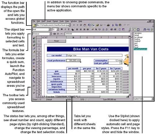 Guided Tour of Calc Use this tutorial to give you a brief introduction to the Calc environment. -
Launch Calc. -
Click cell A1 , type Credit Card Calculator , and press Enter. Cell A2 becomes selected.  -
Click cell A1 again, and in the object bar, change the font size to 24. You can also right-click the cell, choose Format Cells, and in the Cell Attributes window select the Font tab to change the font size. -
Click the number 1 in the gray box of row 1. The entire row is selected.  -
In the object bar, click the Background Color icon, and select a light background color for row 1. 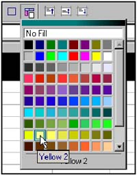 -
In this step you'll enter some row headings. Enter the following text in the corresponding cells, pressing Enter after each entry. (Click each cell to enter the text): (Don't forget the single quote at the beginning. It allows you to use the acronym APR [annual percentage rate] in all capital letters so that Calc doesn't read it as the month April.) -
B4 Monthly Interest -
C4 Starting Balance -
D4 Monthly Payment Notice that not all the text shows in the cells now, as shown in Figure 18-2. Normally you can resize the column widths, have the text wrap in the cells, or both. In this tutorial we'll have you wrap the text. Figure 18-2. Text that is too wide for cells 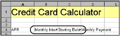 -
Click and hold down the mouse button in cell A4, and drag across the row so that rows A4 through D4 are selected. -
Choose Format > Cells. -
In the Cell Attributes window, click the Alignment tab. -
Select the Line break option and click OK. The text in those cells wraps to show all the text, as shown in Figure 18-3. Figure 18-3. Wrapping text in cells 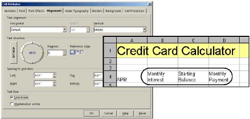 -
Select cells A4 through D4 again. -
In the object bar, click the Bold icon to make the text bold, and click the centered text alignment icon to center the text in the cells.  -
With the cells still highlighted, in the object bar click and hold down the Borders icon, and select the border that shows a line beneath a cell. 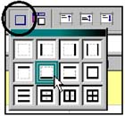 -
Select cell A5 and click the % icon on the object bar. This tells the cell to display a percentage (even though there's no confirmation when you click the icon). Enter the number .18 (don't forget the decimal point). Press the Tab key. -
In cell B5 , click the % icon on the object bar. Now enter the following small formula in the cell, pressing the Tab key afterwards: =A5/12 This formula means divide the contents of cell A5 by 12. What you're doing is figuring a monthly interest rate percentage by dividing the annual percentage rate by 12 months. -
In cell C5 , click the Currency icon. This tells the cell to display a dollar amount. Enter 7000 . This beginning balance is the amount you have charged to your credit card (ouch!). Press the Tab key.  -
In cell D5 , click the Currency icon and enter the number 250 . This is the amount you're going to pay each month. Press Enter. Figure 18-4 shows how your spreadsheet should look so far Figure 18-4. This is how your spreadsheet should look at this point 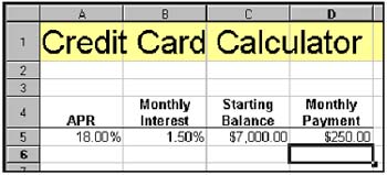 -
In cells A8 through D8 , enter the following text, then make the text bold and centered with a line under the cells (as you did starting in step 11), as shown in Figure 18-5. Figure 18-5. Formatting heading cells  -
In cell A9 , under Payment #, type 1 . -
In cell B9 , under Interest, click the currency icon on the object bar and enter the following formula, then press the Tab key: =$B*$C This formula multiplies the contents of cell B5 by the contents of cell C5 (multiplying the monthly interest rate by the credit card balance). The dollar signs ($) are absolute cell references, which we go into detail about on page 568. -
In cell C9 , under Principal, click the Currency icon and enter the following formula, then press the Tab key: =$D-B9 This formula subtracts the amount of interest you're paying that month from your monthly payment, which gives you the amount of principal subtracted from your overall credit card balance. -
In cell D9 , under Balance, enter the following formula, then press the Tab key: =$C-C9 This subtracts the Principal of the monthly payment from the Starting Balance credit card balance. Your spreadsheet should now look like Figure 18-6. Figure 18-6. This is how your spreadsheet should look at this point 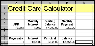 The next steps may seem a little redundant, but they set the stage for the really cool part of the tutorial. -
In cell A10 , the Payment # column, type the number 2 . -
Select cells B10 through D10 and click the Currency icon. -
In cell B10 , in the Interest column, enter the following formula, followed by the Tab key: =D9*$B -
In cell C10 , in the Principal column, enter the following formula followed by the Tab key: =$D-B10 -
In cell D10 , in the Balance column, enter the following formula followed by the Tab key: =D9-C10 Your spreadsheet should now look like Figure 18-7. Figure 18-7. This is how your spreadsheet should look at this point 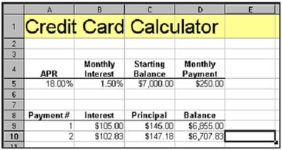 Now comes the fun part. You're going to fill in data about successive payments automatically by clicking and dragging. -
Select cells A10 through D10 . -
On the lower right corner of the selected area, there's a little black square (called the automatic fill handle). Move the mouse pointer on top of that little square. The pointer changes to cross hairs. Click and hold down the mouse button, drag down to row 19, and release the mouse button. The entire selected area fills in with data. Figure 18-8 illustrates this. Figure 18-8. Dragging to fill down 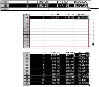 If the new information is all exactly the same, press the F9 key to recalculate the spreadsheet. If you hadn't used absolute and relative cell references in your formulas (discussed on page 568), you would have gotten some crazy results that didn't make sense financially when you filled down. You can fill down even further the same way by selecting cells A19 through D19 and dragging down. You can drag down to where you can see how many payments it's going to take to pay off the credit card. Now let's do something depressing and calculate the total amount of interest you're going to pay based on the number of payments you've filled in. -
In cell E8 , create a column heading called Total Interest Paid , formatted the same way as the other column headings. -
In cell E9 , click the Currency icon and enter the following formula, followed by the Tab key: =SUM(B9:B500) This formula simply adds up all the amounts in the Interest column, from cells B9 to B500 (in case you ever fill down that far), as shown in Figure 18-9. Figure 18-9. Calculating the total interest paid  -
Get out your scissors and cut up your credit card! Post-Tutorial Tips The beauty of spreadsheets is that, if they're set up somewhat correctly (that is, if you set cells up to calculate based on values in other cells, as you did in this exercise), you can change a value in one or two cells to update the values in the entire spreadsheet. For example, if you change the APR percentage in the tutorial spreadsheet (don't forget to start with a decimal point), your entire spreadsheet updates to show what your payment information would be at a different annual interest rate. You can also see different payment scenarios by entering a different monthly payment amount. Make sure you don't try to change spreadsheet information by typing inside cells that have formulas in them. That messes up the whole automated nature of the spreadsheet and can throw off lots of other cell amounts. You can tell if a cell has a formula in it by selecting the cell and looking in the formula bar. Note You can protect yourself from yourself by protecting certain cells you don't want changed, making it so you can't type anything in them. See Protecting Cells From Modification on page 602.
 |